Electromagnetic Simulation Using the FDTD Method with Python

Jennifer E. Houle, Dennis M. Sullivan

• Éditeur: Wiley-IEEE Press
• Année: 2020
• ISBN:
  9781119565840
• Édition: 3
• Sujet: Physical Sciences
• Sous-sujet: Electromagnetism

Provides an introduction to the Finite Difference Time Domain method and shows how Python code can be used to implement various simulations

This book allows engineering students and practicing engineers to learn the finite-difference time-domain (FDTD) method and properly apply it toward their electromagnetic simulation projects. Each chapter contains a concise explanation of an essential concept and instruction on its implementation into computer code. Included projects increase in complexity, ranging from simulations in free space to propagation in dispersive media. This third edition utilizes the Python programming language, which is becoming the preferred computer language for the engineering and scientific community.

Electromagnetic Simulation Using the FDTD Method with Python, Third Edition is written with the goal of enabling readers to learn the FDTD method in a manageable amount of time. Some basic applications of signal processing theory are explained to enhance the effectiveness of FDTD simulation. Topics covered in include one-dimensional simulation with the FDTD method, two-dimensional simulation, and three-dimensional simulation. The book also covers advanced Python features and deep regional hyperthermia treatment planning.

Electromagnetic Simulation Using the FDTD Method with Python:

• Guides the reader from basic programs to complex, three-dimensional programs in a tutorial fashion
• Includes a rewritten fifth chapter that illustrates the most interesting applications in FDTD and the advanced graphics techniques of Python
• Covers peripheral topics pertinent to time-domain simulation, such as Z-transforms and the discrete Fourier transform
• Provides Python simulation programs on an accompanying website

An ideal book for senior undergraduate engineering students studying FDTD, Electromagnetic Simulation Using the FDTD Method with Python will also benefit scientists and engineers interested in the subject.

1
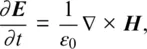
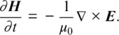
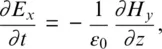
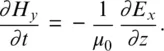
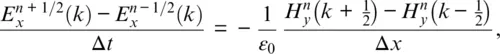
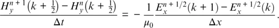
ONE‐DIMENSIONAL SIMULATION WITH THE FDTD METHOD

This chapter provides a step‐by‐step introduction to the finite‐difference time‐domain (FDTD) method, beginning with the simplest possible problem, the simulation of a pulse propagating in free space in one dimension. This example is used to illustrate the FDTD formulation. Subsequent sections lead to formulations for more complicated media.

1.1 ONE‐DIMENSIONAL FREE‐SPACE SIMULATION

The time‐dependent Maxwell’s curl equations for free space are

(1.1a)

(1.1b)

E and H are vectors in three dimensions, so, in general, Eq. (1.1a) and (1.1b) represent three equations each. We will start with a simple one‐dimensional case using only E_x and H_y, so Eq. (1.1a) and (1.1b) become

(1.2a)

(1.2b)

These are the equations of a plane wave traveling in the z direction with the electric field oriented in the x direction and the magnetic field oriented in the y direction.

Taking the central difference approximations for both the temporal and spatial derivatives gives

(1.3a)

(1.3b)

In these two equations, time is specified by the superscripts, that is, n represents a time step, and the time t is t = Δt ⋅ n. Remember, we have to discretize everything for formulation into the computer. The term n + 1 means one time step later. The terms in parentheses represent distance, that is, k is used to calculate the distance z = Δx ⋅ k. (It might seem more sensible to use Δz as the incremental step because in this case we are going in the z direction. However, Δx is so commonly used for a spatial increment that we will use Δx.) The formulation of Eq. (1.3a) and (1.3b) assume that the E and H fields are interleaved in both space and time. H uses the arguments k + 1/2 and k − 1/2 to indicate that the H field values are assumed to be located between the E field values. This is illustrated in Fig. 1.1. Similarly, the n + 1/2 or n − 1/2 superscript indicates that it occurs slightly after o...