![]()
Part One
Foundations of Risk Management
![]()
Chapter 1
Risk Management*
Financial risk management is the process by which financial risks are identified, assessed, measured, and managed in order to create economic value.
Some risks can be measured reasonably well. For those, risk can be quantified using statistical tools to generate a probability distribution of profits and losses. Other risks are not amenable to formal measurement but are nonetheless important. The function of the risk manager is to evaluate financial risks using both quantitative tools and judgment.
As financial markets have expanded over recent decades, the risk management function has become more important. Risk can never be entirely avoided. More generally, the goal is not to minimize risk; it is to take smart risks.
Risk that can be measured can be managed better. Investors assume risk only because they expect to be compensated for it in the form of higher returns. To decide how to balance risk against return, however, requires risk measurement.
Centralized risk management tools such as value at risk (VAR) were developed in the early 1990s. They combine two main ideas. The first is that risk should be measured at the top level of the institution or the portfolio. This idea is not new. It was developed by Harry Markowitz (1952), who emphasized the importance of measuring risk in a total portfolio context.1 A centralized risk measure properly accounts for hedging and diversification effects. It also reflects the fact that equity is a common capital buffer to absorb all risks. The second idea is that risk should be measured on a forward-looking basis, using the current positions.
This chapter gives an overview of the foundations of risk management. Section 1.1 provides an introduction to the risk measurement process, using an illustration. Next, Section 1.2 discusses how to evaluate the quality of risk management processes. Section 1.3 then turns to the integration of risk measurement with business decisions, which is a portfolio construction problem. These portfolio decisions can be aggregated across investors, leading to asset pricing theories that can be used as yardsticks for performance evaluation and for judging risk management and are covered in Section 1.4. Finally, Section 1.5 discusses how risk management can add economic value.
1.1 RISK MEASUREMENT
1.1.1 Example
The first step in risk management is the measurement of risk. To illustrate, consider a portfolio with $100 million invested in U.S. equities. Presumably, the investor undertook the position because of an expectation for profit, or investment growth. This portfolio is also risky, however.
The key issue is whether the expected profit for this portfolio warrants the assumed risk. Thus a trade-off is involved, as in most economic problems. To help answer this question, the risk manager should construct the distribution of potential profits and losses on this investment. This shows how much the portfolio can lose, thus enabling the investor to make investment decisions.
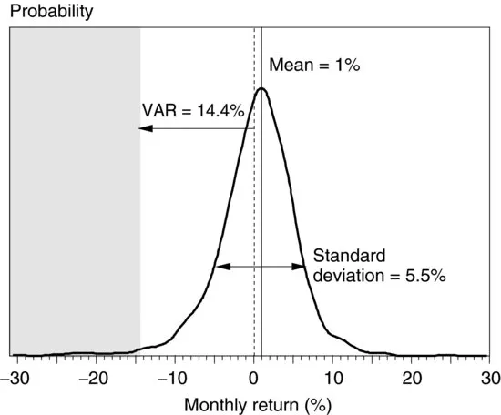
Define Δ P as the profit or loss for the portfolio over a fixed horizon, say the coming month. This must be measured in a risk currency, such as the dollar. This is also the product of the initial investment value P and the future rate of return RP. The latter is a random variable, which should be described using its probability density function. Using historical data over a long period, for example, the risk manager produces Figure 1.1.
This graph is based on the actual distribution of total returns on the S&P 500 index since 1925. The line is a smoothed histogram and does not assume a simplified model such as the normal distribution.
The vertical axis represents the frequency, or probability, of a gain or loss of a size indicated on the horizontal axis. The entire area under the curve covers all of the possible realizations, so should add up to a total probability of 1.
Most of the weight is in the center of the distribution. This shows that it is most likely that the return will be small, whether positive or negative. The tails have less weight, indicating that large returns are less likely. This is a typical characteristic of returns on financial assets. So far, this pattern resembles the bell-shaped curve for a normal distribution.
On the downside, however, there is a substantial probability of losing 10% or more in a month. This cumulative probability is 3%, meaning that in a repeated sample with 100 months, we should expect to lose 10% or more for a total of three months. This risk is worse than predicted by a normal distribution.
If this risk is too large for the investor, then some money should be allocated to cash. Of course, this comes at the expense of lower expected returns.
The distribution can be characterized in several ways. The entire shape is most informative because it could reveal a greater propensity to large losses than to gains. The distribution could be described by just a few summary statistics, keeping in mind that this is an oversimplification. Other chapters offer formal definitions of these statistics.
- The mean, or average return, which is approximately 1% per month. Define this as μ(RP), or μP in short, or even μ when there is no other asset.
- The standard deviation, which is approximately 5.5%. This is often called volatility and is a measure of dispersion around the mean. Define this as σ. This is the square root of the portfolio variance, σ2.
- The value at risk (VAR), which is the cutoff point such that there is a low probability of a greater loss. This is also the percentile of the distribution. Using a 99% confidence level, for example, we find a VAR of 14.4%.
1.1.2 Absolute versus Relative Risk
So far, we have assumed that risk is measured by the dispersion of dollar returns, or in absolute terms. In some cases, however, risk should be measured relative to some benchmark. For example, the performance of an active manager is compared to that of an index such as the S&P 500 index for U.S. equities. Alternatively, an investor may have future liabilities, in which case the benchmark is an index of the present value of liabilities. An investor may also want to measure returns after accounting for the effect of inflation. In all of these cases, the investor is concerned with relative risk.
- Absolute risk is measured in terms of shortfall relative to the initial value of the investment, or perhaps an investment in cash. Using the standard deviation as the risk measure, absolute risk in dollar terms is
- Relative risk is measured relative to a benchmark index B. The deviation is e = RP − RB, which is also known as the tracking error. In dollar terms, this is e × P. The risk is where ω is called tracking error volatility (TEV).
To compare these two approaches, take the case of an active equity portfolio manager who is given the task of beating a benchmark. In the first year, the a...