Analog and Hybrid Computer Programming

Bernd Ulmann

• Publisher: De Gruyter Oldenbourg
• Year: 2020
• ISBN:
  9783110662245
• Edition: 1
• Topic: Technology & Engineering
• Subtopic: Electrical Engineering & Telecommunications
• Index: Technology & Engineering

Analog and hybrid computing recently have gained much interest as analog computers can outperform classical stored-program digital computers in some areas by orders of magnitude. This book gives a thorough introduction to analog and hybrid computer programming by means numerous worked examples from various areas. It is based on a number of introductory and advanced lectures on this topic delivered by the author at several universities.

CHAPTER 1

Introduction

1.1What is an analog computer?

A book about programming analog and hybrid computers may seem like an anachronism in the 21st century – why should one be written and, even more important, why should you read it? As much as analog computers seem to be forgotten, they not only have an interesting and illustrious past but also an exciting and promising future in many application areas such as high performance computing (HPC for short), the field of dynamic systems simulation, education and research, artificial intelligence (biological brains operate, in fact, much like analog computers), and, last but not least, as coprocessors for traditional stored-program digital computers, forming so-called hybrid computers.

From today’s perspective, analog computers are mainly thought of as being museum pieces and their programming paradigm seems archaic at first glance. This impression is as wrong as can be and is mostly caused by the classic patch field or patch panel onto which programs are patched in form of an intricate maze of wires, resembling real spaghetti “code”. . . On reflection, this form of programming is much easier and more intuitive than the algorithmic approach used for stored-program digital computers (which will be just called digital computers from now on to simplify things). Future implementations of analog computers, especially those intended as coprocessors, will probably feature electronic cross-bar switches instead of a patch field. Programming such machines will resemble the programming of a field programmable gate array (FPGA), i. e. a compiler will transforma set of problem equations into a suitable setup of the crossbar-switches, thus configuring the analog computer for the problem to be solved.

The notion of an analog computer has its roots in the Greek word ἀνἀλογον (“analogon”) which lives on in terms like “analogy” and “analogue”. This quite aptly characterizes an analog computer and separates it from today’s digital computers. The latter have a fixed internal structure and are controlled by a program stored in some kind of random access memory.

In contrast, an analog computer has no program memory at all and is programmed by actually changing its structure until it forms an analogue, a model, of a given problem. This approach is in stark contrast to what is taught in programming classes today (apart from those dealing with FPGAs). Problems are not solved in a step-wise (algorithmic) way but instead by connecting the various computing elements of an analog computer in a suitable manner forming a circuit that serves as a model of the problem under investigation. Figures 1.1 and 1.2 illustrate these two fundamentally different approaches to computing. While a classic digital computer works more or less in a sequential fashion, the computing elements of an analog computer work in perfect parallelism with none of the synchronization issues that are often encountered in digital computing.

1.2Direct vs. indirect analogies

When it comes to analogies in general, it is necessary to distinguish between direct and indirect analogies, which depend on the underlying principles of the problems being solved and the analogies used to solve them. In short, a direct analogy has its roots basically in the same physical principles as the corresponding problem, i. e. a soap-bubble being used to model a minimal surface, a metal sheet with heaters and thermocouples to investigate heat-flow patterns etc. If the physical principles underlying the problem and analog computer differ, the computer is called an indirect analog computer.

For the remainder of this book only indirect analogies will be considered, as these are much more versatile in application than their direct counterparts. Typically, such machines are based on analog-electronic computing elements such as summers, integrators, multipliers and the like.

Although it sounds like a contradiction, analog computers can be implemented using purely digital components. Two such types of machine are digital differential analyzers (DDAs) and stochastic computers, examples of which have been built over many years and whilst they enjoy periodic renaissances, they have never entered the mainstream of computing. Programming these machines follows basically the same lines as programming analog-electronic analog computers (simply called analog computers). These digital analog computers will not be discussed further in the book.2

Fig. 1.1. Principle of operation of a stored-program digital computer (see [Truitt et al. 1960, p. 1-40])

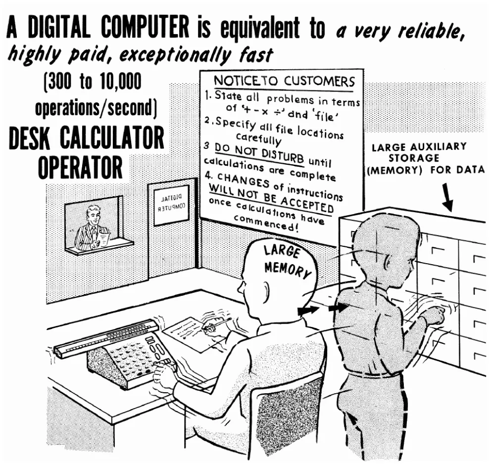
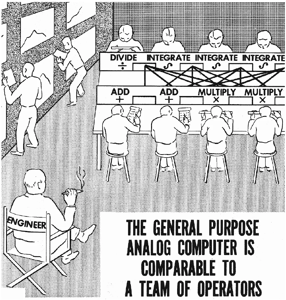
Fig. 1.2. Structure of analog computer (see [TRUITT et al. 1960, p. 1-41])

1.3A short history of analog computing

The idea of analog computing is, of course, much older than today’s predominantly algorithmic approach. In fact, the very first machine that might aptly be called an analog computer is the Antikythera mechanism, a mechanical marvel that was built around 100 B. C. It has been named after the Greek island Aντιϰύθηρα (Antikythera) where its remains were found in a Roman wreck by sponge divers in 1900. At first neglected, the highly corroded lump of gears aroused the interest of DEREK DE SOLLA PRICE, who summarized his scientific findings as follows:3

“It is a bit frightening to know that just before the fall of their great civilization the ancient Greeks had come so close to our age, not only in their thought, but also in their scientific technology.”

Research into this mechanism, which defies all expectations with respect to an ancient computing device, is still ongoing. Its purpose was to calculate sun and moon positions, to predict eclipses and possibly much more. The mechanism consists of more than 30 gears of extraordinary precision yielding a mechanical analogue for the study of celestial mechanics, something that was neither heard of or even thought of for many centuries to come.4

Slide rules can also be regarded as simple analog computers as they allow the execution of multiplication, division, rooting etc. by shifting of (mostly) logarithmic scales against each other. Nevertheless, these are rather specialized analog computers, just as planimeters, which were (and to some extent still are) used to measure the area of closed figures, a task that frequently occurs in surveying but also in all branches of natural science and engineering.

Things became more interesting in the 19th and early 20th century with the development and application of practical mechanical integrators. Based on such developments, WILLIAM THOMSON, later Lord KELVIN, developed the concept of a machine capable of solving differential equations. Although no usable computer evolved from this, his ideas proved very fruitful. Specifically, his approach to programming such machines is still used today and called the KELVIN feedback technique.5

Fig. 1.3. VANNEVAR BUSH’s mechanical differential analyzer (source: [Meccano 1934, p. 443])

Figure 1.3 shows a mechanical analog computer, called a differential analyzer. On both sides of the long table-like structure in the middle of the picture, various computing elements such as integrators (discernible by the small horizontal disks), differential gears, plotter tables etc. can be seen. The elongated structure in the middle is the actual interconnect of these computing devices which consists of a myriad of axles and gears. Programming such a machine was a cumbersome and time consuming process as the interconnection structure had to be more or less completely dismantled and rebuilt every time the machine was configured to solve the differential equations which describe the new problem.

Figure 1.4 shows a simple setup of a differential analyzer to integrate a function given in graphical form. A central motor, shown on the ...

Table of contents

• Cover
• Title Page
• Copyright
• Dedication
• Acknowledgments and disclaimer
• Contents
• 1 Introduction
• 2 Computing elements
• 3 Analog computer operation
• 4 Basic programming
• 5 Special functions
• 6 Examples
• 7 Hybrid computing
• 8 Summary and outlook
• A Solving the heat equation with a passive network
• B The Laplace transform
• C Mikusiński operational calculus
• D An oscilloscope multiplexer
• E A log() function generator
• F A sine/cosine generator
• G A simple joystick interface
• H The Analog Paradigm bus system
• I HyCon commands
• Bibliography
• Index