CREI Lectures in Macroeconomics

Robert Shimer

• Publisher: Princeton University Press
• Year: 2010
• ISBN:
  9781400835232
• Topic: Economics
• Subtopic: Labour Economics
• Index: Economics

Labor Markets and Business Cycles integrates search and matching theory with the neoclassical growth model to better understand labor market outcomes. Robert Shimer shows analytically and quantitatively that rigid wages are important for explaining the volatile behavior of the unemployment rate in business cycles.
The book focuses on the labor wedge that arises when the marginal rate of substitution between consumption and leisure does not equal the marginal product of labor. According to competitive models of the labor market, the labor wedge should be constant and equal to the labor income tax rate. But in U.S. data, the wedge is strongly countercyclical, making it seem as if recessions are periods when workers are dissuaded from working and firms are dissuaded from hiring because of an increase in the labor income tax rate. When job searches are time consuming and wages are flexible, search frictions--the cost of a job search--act like labor adjustment costs, further exacerbating inconsistencies between the competitive model and data. The book shows that wage rigidities can reconcile the search model with the data, providing a quantitatively more accurate depiction of labor markets, consumption, and investment dynamics.
Developing detailed search and matching models, Labor Markets and Business Cycles will be the main reference for those interested in the intersection of labor market dynamics and business cycle research.

1

The Labor Wedge

Throughout this book, I study the interaction of optimizing households and firms in a closed economy. I begin in this chapter by developing a competitive, representative-agent version of the model. The chapter has two objectives. First, I introduce much of the notation that I rely on throughout the book. Because of this, I include details in this chapter that are not really necessary for the second, more substantive objective: I use the model to measure and analyze the behavior of the labor wedge, the wedge between the marginal rate of substitution of consumption for leisure and the marginal product of labor. I confirm the well-known result that the labor wedge tends to rise during recessions, so the economy behaves as if there is a countercyclical tax on labor. The remainder of the book explores whether extending the model to incorporate labor market search frictions can explain the behavior of the labor wedge.

I start the chapter by laying out the essential features of the model: optimizing households, optimizing firms, a government that sets taxes and spending, and equilibrium conditions that link the various agents. In section 1.2, I use pieces of the model to derive a static equation that relates hours worked, the consumption–output ratio, and the labor wedge. Section 1.3 discusses how I measure the first two concepts and uses these measures to calculate the implied behavior of the labor wedge in the United States. I establish the main substantive result: that the labor wedge rose strongly during every recession since 1970. I show the robustness of my results to alternative specifications of preferences in section 1.4 and discuss the possibility that the results are driven by preference shocks in section 1.5. I finish the chapter with a brief discussion in section 1.6 on the empirical relationship between the fluctuations in hours, which I analyze here, and fluctuations in employment and unemployment, which are the main topic of subsequent chapters.

1.1 A Representative-Agent Model

I denote time by t = 0, 1, 2, . . . and the state of the economy at time t by s_t. Let s^t = {s₀, s₁, . . . , s_t} denote the history of the economy and Π(s^t) denote the time-0 belief about the probability of observing an arbitrary history s^t through time t. Exogenous variables like aggregate productivity, government spending, and distortionary tax rates may depend on the history s^t. At date 0, there is an initial capital stock k₀ ≡ k(s⁰) and an initial stock of government debt b₀ ≡ b(s⁰). The capital stock is owned by firms, while households hold the debt and own the firms.

Households

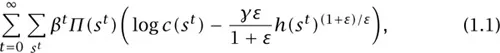
A representative household is infinitely lived and has preferences over history-s^t consumption c(s^t) and history-s^t hours of work h(s^t). To start, I assume that preferences are ordered by the utility function

where β ∈ (0, 1) is the discount factor,

measures the disutility of working, and, as I show below, ε > 0 is the Frisch (constant marginal utility of wealth) elasticity of labor supply.

This formulation implies that preferences are additively separable over time and across states of the world. It also implies that preferences are consistent with balanced growth—doubling a household’s initial assets and its income in every state of the world doubles its consumption but does not affect its labor supply. This is consistent with the absence of a secular trend in hours worked per household, at least in the United States (Aguiar and Hurst 2007; Ramey and Francis 2009). I maintain both of these assumptions throughout this book. The formulation also imposes that the marginal utility of consumption is independent of the worker’s leisure. This restriction is more questionable and so I relax it in section 1.4 below.

The household chooses a sequence for consumption and hours of work to maximize utility subject to a single lifetime budget constraint,

The household has initial assets a₀ = a(s⁰). In addition,

is the labor income tax rate,

is the hourly wage rate, and T(s^t) is a lump-sum transfer in history s^t, all denominated in contemporaneous units of consumption.¹ Thus

represents consumption in excess of after-tax labor income and transfers, which is discounted back to time 0 according to the intertemporal price q₀ (s^t). That is, q₀ (s^t) represents the cost in history s⁰ of purchasing one unit of consumption in history s^t, denominated in units of history-s⁰ consumption. Put differently, q₀(s^t) is the history-s⁰ price of an Arrow–Debreu security that pays one unit of consumption in history s^t and nothing otherwise. Equation (1.2) states that the household’s net purchase of Arrow–Debreu securities in history s⁰ must be equal to its initial assets a₀.

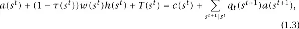
It will be useful to define the assets of the household, following history s^t, as

where the notation s^t′|s^t indicates that the summation is taken over histories of s^t′ that are continuation histories of s^t, i.e., s^t′ ≡ {s^t, s_t+1, s_t+2, . . . , s_t′} for some states {s_t+1, s_t+2, . . . , s_t′}. Then q_t(s^t′) is the price of a unit of consumption in history s^t′ = {s^t, s_t+1, s_t+2, . . . , s_t′} paid in units of history-s^t consumption. The absence of arbitrage opportunities requires that q₀(s^t)q_t(s^t+1) = q₀(s^t+1) for all s^t and for all s^t+1 ≡ {s^t, s_t+1}. Equivalently, the lifetime budget constraint implies a sequence of intertemporal budget constraints,

so assets plus labor income plus transfers in history s^t is equal to consumption plus purchases of assets in continuation histories s^t+1.

Firms

The representative firm owns the capital stock k₀ = k(s⁰) and has access to a Cobb–Douglas production function, producing gross output z(s^t)k(s^t)^αh^d(s^t)^1-α in history s^t, where z(s^t) is history-contingent total factor pro...

Table of contents

• Cover
• Half title
• Title
• Copyright
• Contents
• Introduction
• Preface
• 1 The Labor Wedge
• 2 Benchmark Search Model: Neutrality
• 3 Real Effects of Productivity Shocks
• 4 Rigid Wages
• 5 Looking Ahead
• Appendix A. Data
• References
• Author Index