Continuum Mechanics

A. J. M. Spencer

• Verlag: Dover Publications
• Jahr: 2012
• ISBN:
  9780486139470
• Thema: Physical Sciences
• Thema: Physics

The mechanics of fluids and the mechanics of solids represent the two major areas of physics and applied mathematics that meet in continuum mechanics, a field that forms the foundation of civil and mechanical engineering. This unified approach to the teaching of fluid and solid mechanics focuses on the general mechanical principles that apply to all materials. Students who have familiarized themselves with the basic principles can go on to specialize in any of the different branches of continuum mechanics. This text opens with introductory chapters on matrix algebra, vectors and Cartesian tensors, and an analysis of deformation and stress. Succeeding chapters examine the mathematical statements of the laws of conservation of mass, momentum, and energy as well as the formulation of the mechanical constitutive equations for various classes of fluids and solids. In addition to many worked examples, this volume features a graded selection of problems (with answers, where appropriate). Geared toward undergraduate students of applied mathematics, it will also prove valuable to physicists and engineers. 1992 edition.

1

Introduction

1.1 Continuum mechanics

Modern physical theories tell us that on the microscopic scale matter is discontinuous; it consists of molecules, atoms and even smaller particles. However, we usually have to deal with pieces of matter which are very large compared with these particles; this is true in everyday life, in nearly all engineering applications of mechanics, and in many applications in physics. In such cases we are not concerned with the motion of individual atoms and molecules, but only with their behaviour in some average sense. In principle, if we knew enough about the behaviour of matter on the microscopic scale it would be possible to calculate the way in which material behaves on the macroscopic scale by applying appropriate statistical procedures. In practice, such calculations are extremely difficult; only the simplest systems can be studied in this way, and even in these simple cases many approximations have to be made in order to obtain results. Consequently, our knowledge of the mechanical behaviour of materials is almost entirely based on observations and experimental tests of their behaviour on a relatively large scale.

Continuum mechanics is concerned with the mechanical behaviour of solids and fluids on the macroscopic scale. It ignores the discrete nature of matter, and treats material as uniformly distributed throughout regions of space. It is then possible to define quantities such as density, displacement, velocity, and so on, as continuous (or at least piecewise continuous) functions of position. This procedure is found to be satisfactory provided that we deal with bodies whose dimensions are large compared with the characteristic lengths (for example, interatomic spacings in a crystal, or mean free paths in a gas) on the microscopic scale. The microscopic scale need not be of atomic dimensions; we can, for example, apply continuum mechanics to a granular material such as sand, provided that the dimensions of the region considered are large compared with those of an individual grain. In continuum mechanics it is assumed that we can associate a particle of matter with each and every point of the region of space occupied by a body, and ascribe field quantities such as density, velocity, and so on, to these particles. The justification for this procedure is to some extent based on statistical mechanical theories of gases, liquids and solids, but rests mainly on its success in describing and predicting the mechanical behaviour of material in bulk.

Mechanics is the science which deals with the interaction between force and motion. Consequently, the variables which occur in continuum mechanics are, on the one hand, variables related to forces (usually force per unit area or per unit volume, rather than force itself) and, on the other hand, kinematic variables such as displacement, velocity and acceleration. In rigid-body mechanics, the shape of a body does not change, and so the particles which make up a rigid body may only move relatively to one another in a very restricted way. A rigid body is a continuum, but it is a very special, idealized and untypical one. Continuum mechanics is more concerned with deformable bodies, which are capable of changing their shape. For such bodies the relative motion of the particles is important, and this introduces as significant kinematic variables the spatial derivatives of displacement, velocity, and so on.

The equations of continuum mechanics are of two main kinds. Firstly, there are equations which apply equally to all materials. They describe universal physical laws, such as conservation of mass and energy. Secondly, there are equations which describe the mechanical behaviour of particular materials; these are known as constitutive equations.

The problems of continuum mechanics are also of two main kinds. The first is the formulation of constitutive equations which are adequate to describe the mechanical behaviour of various particular materials or classes of materials. This formulation is essentially a matter for experimental determination, but a theoretical framework is neeeded in order to devise suitable experiments and to interpret experimental results. The second problem is to solve the constitutive equations, in conjunction with the general equations of continuum mechanics, and subject to appropriate boundary conditions, to confirm the validity of the constitutive equations and to predict and describe the behaviour of materials in situations which are of engineering, physical or mathematical interest. At this problem-solving stage the different branches of continuum mechanics diverge, and we leave this aspect of the subject to more comprehensive and more specialized texts.

2

Introductory matrix algebra

2.1 Matrices

In this chapter we summarize some useful results from matrix algebra. It is assumed that the reader is familiar with the elementary operations of matrix addition, multiplication, inversion and transposition. Most of the other properties of matrices which we will present are also elementary, and some of them are quoted without proof. The omitted proofs will be found in standard texts on matrix algebra.

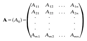
An m x n matrix A is an ordered rectangular array of mn elements. We denote

(2.1)

so that A_ij is the element in the ith row and the jth column of the matrix A. The index i takes values 1, 2, . . . , m, and the index j takes values 1, 2, . . . , n. In continuum mechanics the matrices which occur are usually either 3 x 3 square matrices, 3 × 1 column matrices or 1 x 3 row matrices. We shall usually denote 3 x 3 square matrices by bold-face roman capital letters (A, B, C, etc.) and 3 x 1 column matrices by bold-face roman lower-case letters (a, b, c, etc.). A 1 x 3 row matrix will be treated as the transpose of a 3 x 1 column matrix (a^T, b^T, c^T, etc.). Unless otherwise stated, indices will take the values 1, 2 and 3, although most of the results to be given remain true for arbitrary ranges of the indices.

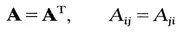
A square matrix A is symmetric if

(2.2)

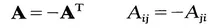
and anti-symmetric if

(2.3)

where A^T denotes the transpose of A.

The 3 x 3 unit matrix is denoted by I, and its elements by δ_ij....

Inhaltsverzeichnis

• Title Page
• Copyright Page
• Table of Contents
• Preface
• 1 - Introduction
• 2 - Introductory matrix algebra
• 3 - Vectors and cartesian tensors
• 4 - Particle kinematics
• 5 - Stress
• 6 - Motions and deformations
• 7 - Conservation laws
• 8 - Linear constitutive equations
• 9 - Further analysis of finite deformation
• 10 - Non-linear constitutive equations
• 11 - Cylindrical and spherical polar coordinates
• Appendix - Representation theorem for an isotropic tensor function of a tensor
• Answers
• Further reading
• Index