The Analysis of Time Series

An Introduction with R

Chris Chatfield, Haipeng Xing

• Editorial: Chapman and Hall/CRC
• Año: 2019
• ISBN:
  9781498795661
• Edición: 7
• Categoría: Mathematics
• Categoría: Probability & Statistics

This new edition of this classic title, now in its seventh edition, presents a balanced and comprehensive introduction to the theory, implementation, and practice of time series analysis. The book covers a wide range of topics, including ARIMA models, forecasting methods, spectral analysis, linear systems, state-space models, the Kalman filters, nonlinear models, volatility models, and multivariate models.

Chapter 1

Introduction

A time series is a collection of observations made sequentially through time. Examples occur in a variety of fields, ranging from economics to engineering, and methods of analysing time series constitute an important area of statistics.

1.1Some Representative Time Series

We begin with some examples of the sort of time series that arise in practice.

Economic and financial time series

Many time series are routinely recorded in economics and finance. Examples include share prices on successive days, export totals in successive months, average incomes in successive months, company profits in successive years and so on.

The classic Beveridge wheat price index series consists of the average wheat price in nearly 50 places in various countries measured in successive years from 1500 to 1869 (Beveridge, 1921). This series is of particular interest to economics historians, and is available in many places (e.g. in the tseries package of R). Figure 1.1 shows this series and some apparent cyclic behaviour can be seen. The trend of the series will be studied in Section 2.5.2.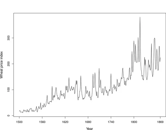

Figure 1.1The Beveridge wheat price annual index series from 1500 to 1869.

To plot the data using the R statistical package, you can load the data bev in the tseries package and plot the time series (the > below are prompts):

 > library(tseries) # load the library > data(bev) # load the dataset > plot(bev, xlab="Year", ylab="Wheat price index", xaxt="n") > x.pos<-c(1500, 1560, 1620, 1680, 1740, 1800, 1869)  # define x-axis labels > axis(1, x.pos, x.pos) 

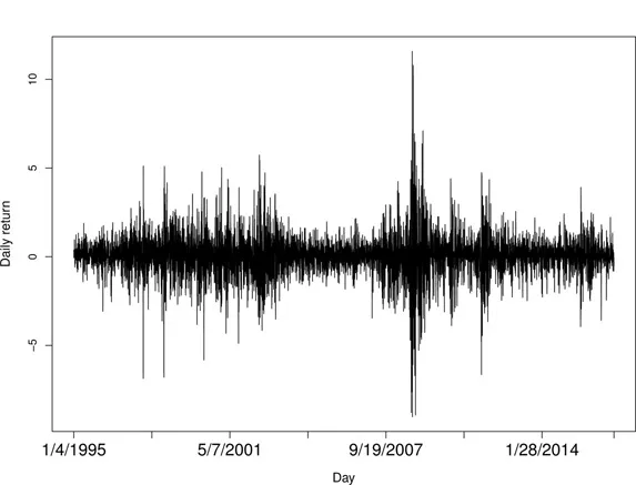
As an example of financial time series, Figure 1.2 shows the daily returns (or percentage change) of the adjusted closing prices of the Standard & Poor’s 500 (S&P500) Index from January 4, 1995 to December 30, 2016. The data shown in Figure 1.2 are typical of return data. The mean of the return series seems to be stable with an average return of approximately zero, but the volatility of data changes over time. This series will be analyzed in Chapter 12.

Figure 1.2Daily returns of the adjusted closing prices of the S&P500 index from January 4, 1995 to December 30, 2016.

To reproduce Figure 1.2 in R, suppose you save the data as sp500_ret_1995-2016.csv in the directory mydata. Then you can use the following command to read the data and plot the time series.

 > sp500<-read.csv("mydata/sp500_ret_1995-2016.csv") > n<-nrow(sp500) > x.pos<-c(seq(1,n,800),n) > plot(sp500{\$}Return, type="l", xlab="Day",  ylab="Daily return", xaxt="n") > axis(1, x.pos, sp500{\$}Date[x.pos]) 

Physical time series

Many types of time series occur in the physical sciences, particularly in meteorology, marine science and geophysics. Examples are rainfall on successive days, and air temperature measured in successive hours, days or months. Figure 1.3 shows the average air temperature in Anchorage, Alaska in the United States in successive months over a 16-year period. The series can be downloaded from the U.S. National Centers for Environmental Information (https://www.ncdc.noaa.gov/cag/). Seasonal fluctuations can be clearly seen in the series.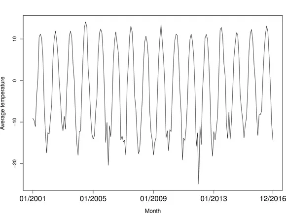

Figure 1.3Monthly average air temperature (deg C) in Anchorage, Alaska, the United States, in successive months from 2001 to 2016.

Some mechanical recorders take measurements continuously and produce a continuous trace rather than observations at discrete intervals of time. For example, in some laboratories it is important to keep temperature and humidity as constant as possible and so devices are installed to measure these variables continuously. Action may be taken when the trace goes outside pre-specified limits. Visual examination of the trace may be adequate for many purposes, but, for more detailed analysis, it is customary to convert the continuous trace to a series in discrete time by sampling the trace at appropriate equal intervals of time. The resulting analysis is more straightforward and can readily be handled by standard time series software.

Marketing time series

The analysis of time series arising in marketing is an important problem in commerce. Observed variables could include sales figures in successive weeks or months, monetary receipts, advertising costs and so on. As an example, Figure 1.4 shows the domestic sales of Australian fortified wine by winemakers in successive quarters over a 30-year period, which are available at the Australian Bureau of Statistics (http://www.abs.gov.au/AUSSTATS/). This series will be analysed in Sections 4.8 and 4.9. Note the trend and seasonal variation which is typical of sales data. It is often important to forecast future sales so as to plan production. It may also be of interest to examine the relationship between sales and other time series such as advertising expenditure.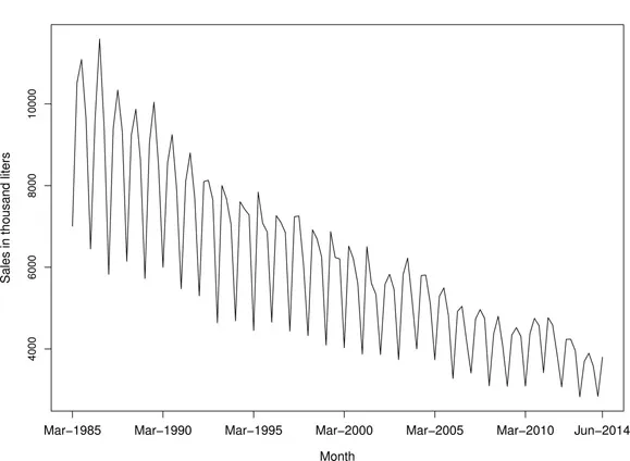

Figure 1.4Domestic sales (unit: thousand liters) of Australian fortified wine by winemakers in successive quarters from March 1985 to June 2014.

Demographic time series

Various time series occur in the study of population change. Examples include the total population of Canada measured annually, and monthly birth totals in England. Figure 1.5 shows the total population and crude birth rate (per 1,000 people) for the United States from 1965 to 2015. The data are available at the U.S. Federal Reserve Bank of St. Louis (https://fred.stlouisfed.org/). Demographers want to predict changes in population for as long as 10 or 20 years into the future, and are helped by the slowly changing structure of a human population. Standard time series methods can be applied to study this problem.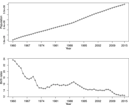

Figure 1.5Total population and birth rate (per 1,000 people) for the United States from 1965 to 2015.

To reproduce Figure 1.5 in R, you can use the following command to read the data and plot the time series.

 > pop<-read.csv("mydata/US_pop_birthrate.csv", header=T) > x.pos<-c(seq(1, 56, 7), 56) > x.label<-c(seq(1960, 2009, by=7), 2015) > par(mfrow=c(2,1), mar=c(3,4,3,4)) > plot(pop[,2], type="l", xlab="", ylab="", xaxt="n") > points(pop[,2]) > axis(1, x.pos, x.label, cex.axis=1.2) > title(xlab="Year", ylab="Population", line=2, cex.lab=1.2) > plot(pop[,3], type="l", xlab="", ylab="", xaxt="n") > points(pop[,3]) > axis(1, x.pos, x.label, cex.axis=1.2) > title(xlab="Year", ylab="Birth rates", line=2, cex.lab=1.2) 

Process control data

In process control, a problem is to detect changes in the performance of a manufacturing process by measuring a variable, which shows the quality of the process. These measurements can be plotted against time as in Figure 1.6. When the measurements stray too far from some target value, appropriate ...