Financial Risk Forecasting

The Theory and Practice of Forecasting Market Risk with Implementation in R and Matlab

Jon Danielsson

• Éditeur: Wiley
• Année: 2011
• ISBN:
  9781119977117
• Édition: 1
• Sujet: Negocios y empresa
• Sous-sujet: Seguros

Financial Risk Forecasting is a complete introduction to practical quantitative risk management, with a focus on market risk. Derived from the authors teaching notes and years spent training practitioners in risk management techniques, it brings together the three key disciplines of finance, statistics and modeling (programming), to provide a thorough grounding in risk management techniques.

Written by renowned risk expert Jon Danielsson, the book begins with an introduction to financial markets and market prices, volatility clusters, fat tails and nonlinear dependence. It then goes on to present volatility forecasting with both univatiate and multivatiate methods, discussing the various methods used by industry, with a special focus on the GARCH family of models. The evaluation of the quality of forecasts is discussed in detail. Next, the main concepts in risk and models to forecast risk are discussed, especially volatility, value-at-risk and expected shortfall. The focus is both on risk in basic assets such as stocks and foreign exchange, but also calculations of risk in bonds and options, with analytical methods such as delta-normal VaR and duration-normal VaR and Monte Carlo simulation. The book then moves on to the evaluation of risk models with methods like backtesting, followed by a discussion on stress testing. The book concludes by focussing on the forecasting of risk in very large and uncommon events with extreme value theory and considering the underlying assumptions behind almost every risk model in practical use – that risk is exogenous – and what happens when those assumptions are violated.

Every method presented brings together theoretical discussion and derivation of key equations and a discussion of issues in practical implementation. Each method is implemented in both MATLAB and R, two of the most commonly used mathematical programming languages for risk forecasting with which the reader can implement the models illustrated in the book.

The book includes four appendices. The first introduces basic concepts in statistics and financial time series referred to throughout the book. The second and third introduce R and MATLAB, providing a discussion of the basic implementation of the software packages. And the final looks at the concept of maximum likelihood, especially issues in implementation and testing.

The book is accompanied by a website - www.financialriskforecasting.com – which features downloadable code as used in the book.

1
Financial markets, prices and risk

The focus of this chapter is on the statistical techniques used for analyzing prices and returns in financial markets. The concept of a stock market index is defined followed by a discussion of prices, returns and volatilities. Volatility clusters, the fat-tailed property of financial returns and observed sharp increases in correlations between assets during periods of financial turmoil (i.e., nonlinear dependence) will also be explored.

Various statistical techniques are introduced and used in this chapter for the analysis of financial returns. While readers may have seen these techniques before, Appendix A contains an introduction to basic statistics and time series methods for financial applications. The most common statistical methods presented in this chapter are implemented in the two programming languages discussed in this book: R and Matlab. These languages are discussed in more detail in Appendix B for R and Appendix C for Matlab.

We illustrate the application of statistical methods by using observed stock market data, the S&P 500 for univariate methods and a portfolio of US stocks for multivariate methods. The data can be downloaded from sources such as finance.yahoo.com directly within R and Matlab, as demonstrated by the source code in this chapter.

A key conclusion from this chapter is that we are likely to measure risk incorrectly by using volatility because of the presence of volatility clusters, fat tails and nonlinear dependence. This impacts on many financial applications, such as portfolio management, asset allocation, derivatives pricing, risk management, economic capital and financial stability.

The specific notation used in this chapter is:

T	Sample size
t = 1, …, T	A particular observation period (e.g., a day)
Pt	Price at time t
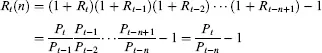
	Simple return
	Continuously compounded return
yt	A sample realization of Yt
σ	Unconditional volatility
σt	Conditional volatility
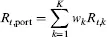
K	Number of assets
ν	Degrees of freedom of the Student-t
t	Tail index

1.1 PRICES, RETURNS AND STOCK INDICES

1.1.1 Stock indices

A stock market index shows how a specified portfolio of share prices changes over time, giving an indication of market trends. If an index goes up by 1%, that means the total value of the securities which make up the index has also increased by 1% in value.

Usually, the index value is described in terms of “points”—we frequently hear statements like “the Dow dropped 500 points today”. The points by themselves do not tell us much that is interesting; the correct way to interpret the value of an index is to compare it with a previous value. One key reason so much attention is paid to indices today is that they are widely used as benchmarks to evaluate the performance of professionally managed portfolios such as mutual funds.

There are two main ways to calculate an index. A price-weighted index is an index where the constituent stocks are weighted based on their price. For example, a stock trading at $100 will make up 10 times more of the total index than a stock trading at $10. However, such an index will not accurately reflect the evolution of underlying market values because the $100 stock might be that of a small company and the $10 stock that of a large company. A change in the price quote of the small company will thus drive the price-weighted index while combined market values will remain relatively constant without changes in the price of the large company. The Dow Jones Industrial Average (DJIA) and the Nikkei 225 are examples of price-weighted stock market indices.

By contrast, the components of a value-weighted index are weighted according to the total market value of their outstanding shares. The impact of a component's price change is therefore proportional to the issue's overall market value, which is the product of the share price and the number of shares outstanding. The weight of each stock constantly shifts with changes in a stock's price and the number of shares outstanding, implying such indices are more informative than price-weighted indices.

Perhaps the most widely used index in the world is the Standard & Poor 500 (S&P 500) which captures the top-500 traded companies in the United States, representing about 75% of US market capitalization. No asset called S&P 500 is traded on financial markets, but it is possible to buy derivatives on the index and its volatility VIX. For the Japanese market the most widely used value-weighted index is the TOPIX, while in the UK it is the FTSE.

1.1.2 Prices and returns

We denote asset prices by P_t, where the t usually refers to a day, but can indicate any frequency (e.g., yearly, weekly, hourly). If there are many assets, each asset is indicated by P_t,k = P_time,asset, and when referring to portfolios we use the subscript “port”. Normally however, we are more interested in the return we make on an investment—not the price itself.

Definition 1.1 (Returns) The relative change in the price of a financial asset over a given time interval, often expressed as a percentage.

Returns also have more attractive statistical properties than prices, such as stationarity and ergodicity. There are two types of returns: simple and compound. We ignore the dividend component for simplicity.

Definition 1.2 (Simple returns) A simple return is the percentage change in prices, indicated by R:

Often, we need to convert daily returns to monthly or annual returns, or vice versa. A multiperiod (n-period) return is given by:

where R_t(n) is the return over the most recent n-periods from date t – n to t.

A convenient advantage of simple returns is that the return on a portfolio, R_t,port, is simply the weighted sum of the returns of individual assets:

where K is the number of assets; and w_k is the portfolio weight of asset i. An alternative return measure is continuously compounded returns.

Definition 1.3 (Continuously compounded returns) Th...