Predicting Presidential Elections and Other Things, Second Edition

Ray Fair

• Éditeur: Stanford Economics and Finance
• Année: 2011
• ISBN:
  9780804778022
• Édition: 2
• Sujet: Economics
• Sous-sujet: Econometrics

"It's the economy, stupid, " as Democratic strategist James Carville would say. After many years of study, Ray C. Fair has found that the state of the economy has a dominant influence on national elections. Just in time for the 2012 presidential election, this new edition of his classic text, Predicting Presidential Elections and Other Things, provides us with a look into the likely future of our nation's political landscape—but Fair doesn't stop there.

Fair puts other national issues under the microscope as well—including congressional elections, Federal Reserve behavior, and inflation. In addition he covers topics well beyond today's headlines, as the book takes on questions of more direct, personal interest such as wine quality, predicting football games, and aging effects in baseball. Which of your friends is most likely to have an extramarital affair? How important is class attendance for academic performance in college? How fast can you expect to run a race or perform some physical task at age 55, given your time at age 30? Read Predicting Presidential Elections and Other Things and find out!

As Fair works his way through an incredibly broad range of questions and topics, he teaches and delights. The discussion that underlies each chapter topic moves from formulating theories about real world phenomena to lessons on how to analyze data, test theories, and make predictions. At the end of this book, readers will walk away with more than mere predictions. They will have learned a new approach to thinking about many age-old concerns in public and private life, and will have a myriad of fun facts to share.

1 It’s the Economy, Stupid

Election night at midnight:

Boy Bryan’s defeat.

Defeat of western silver.

Defeat of the wheat.

Victory of letterfiles

And plutocrats in miles

With dollar signs upon their coats,

Diamond watchchains on their vests and spats on their feet.

Vachel Lindsay, from Bryan, Bryan, Bryan, Bryan

A common pastime in the United States every four years is predicting presidential elections. Polls are taken almost daily in the year of an election, and there are Web sites that allow betting on elections.

Some of the more interesting footnotes to presidential elections concern large errors that were made in predicting who would win. In 1936, the Literary Digest predicted a victory for Republican Alfred Landon over Democrat Franklin Roosevelt by a fairly large margin, when in fact Roosevelt won election to a second term by a landslide. The Literary Digest polled more than 2 million people, so the sample size was huge, but the sample was selected from telephone directories and automobile registrations, which overrepresented wealthy and urban voters, more of whom supported Landon. In addition, the response rate was higher for voters who supported Landon. The Literary Digest never really recovered from this error, and it ceased publication in 1938.

Another famous error was made by the Chicago Tribune in 1948, when it ran the headline “Dewey Wins.” After it became clear that Thomas Dewey had lost, a smiling Harry Truman was photographed holding up the headline.

A more recent large error was made in June 1988, when most polls were predicting Michael Dukakis beating George Bush by about 17 percentage points. A few weeks later, the polls began predicting a Bush victory, which turned out to be correct.

While interesting in their own right, polls are limited in helping us understand what motivates people to vote the way they do. Most polls simply ask people their voting plans, not how or why they arrived at these plans. We must go beyond simple polling results to learn about the factors that influence voting behavior. This is where tools of the social sciences and statistics can be of help.

A Theory of Voting Behavior

To examine the question of why people vote the way they do, we begin with a theory. Consider a person entering a voting booth and deciding which lever to pull for president. Some people are dyed-in-the-wool Republicans and always vote for the Republican candidate. Conversely, others are dyed-in-the-wool Democrats and always vote Democratic. For some, one issue, such as abortion or gun control, dominates all others, and they always vote for the candidate on their side of the issue. For these people, there is not much to explain. One could try to explain why someone became a staunch Republican or Democrat or focused on only one issue, but this is not the main concern here. Of concern here are all the other voters, whom we will call swing voters. Swing voters are those without strong ideological ties and whose views about which party to vote for may change from election to election. For example, Missouri is considered a swing state (that is, a state with many swing voters). It sometimes votes Democratic and sometimes Republican. Massachusetts, on the other hand, almost always votes Democratic, regardless of the state of the economy or anything else, and Idaho almost always votes Republican. The percentage of swing voters in these two states is much smaller than the percentage in Missouri.

What do swing voters think about when they enter the booth? One theory is that swing voters think about how well off financially they expect to be in the future under each candidate and vote for the candidate under whom they expect to be better off. If they expect that their financial situation will be better off under the Democratic candidate, they vote for him or her; otherwise, they vote for the Republican candidate. This is the theory that people “vote their pocketbooks.” The theory need not pertain to all voters, but to be of quantitative interest, it must pertain to a fairly large number.

The Clinton presidential campaign in 1992 seemed aware that there may be something to this theory. In campaign headquarters in Little Rock, Arkansas, James Carville hung up a sign that said, “It’s the Economy, Stupid”—hence the title of this chapter.

The theory as presented so far is hard to test because we do not generally observe voters’ expectations of their future well-being. We must add to the theory an assumption about what influences these expectations. We will assume that the recent performance of the economy at the time of the election influences voters’ expectations of their own future well-being. If the economy has been doing well, voters take this as a positive sign about their future well-being under the incumbent party. Conversely, if the economy has been doing poorly, voters take this as a negative sign. The theory and this assumption then imply that when the economy is doing well, voters tend to vote for the incumbent party, and when the economy is doing poorly, they tend to vote for the opposition party.

We now have something that can be tested. Does the incumbent party tend to do well when the economy is good and poorly when the economy is bad? Let’s begin by taking as the measure of how the economy is doing the growth rate of output per person (real per capita gross domestic product [GDP]) in the year of the election. Let’s also use as the measure of how well the incumbent party does in an election the percentage of the two-party vote that it receives. For example, in 1996, the growth rate was 3.3 percent, and the incumbent party candidate (Bill Clinton) got 54.7 percent of the combined Democratic and Republican vote (and won—over Bob Dole). In 2008, the growth rate was –2.3 percent, and the incumbent party candidate (John McCain) got 46.3 percent of the combined two-party vote (and lost—to Barack Obama). (The reasons for using the two-party vote will be explained later.)

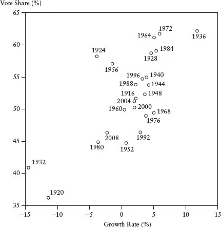
Figure 1-1 is a graph of the incumbent party vote share plotted against the growth rate for the 24 elections between 1916 and 2008. The incumbent party vote share is on the vertical axis, and the growth rate is on the horizontal axis. According to the above theory, there should be a positive relationship between the two: when the growth rate is high, the vote share should be high, and vice versa.

FIGURE 1-1 Incumbent party vote share graphed against the growth rate of the economy

Two observations that stand out in Figure 1-1 are the elections of 1932 and 1936. In 1932, the incumbent party’s candidate (Herbert Hoover) got 40.9 percent of the two-party vote, a huge defeat in a year when the growth rate of the economy was –14.6 percent. (Yes, that’s a minus sign!) In 1936, the incumbent party’s candidate (Franklin Roosevelt) got 62.2 percent of the two-party vote, a huge victory in a year when the growth rate of the economy was an exceptionally strong 11.8 percent. (Although 1936 was in the decade of the Great Depression, the economy actually grew quite rapidly in that year.)

Figure 1-1 shows that there does appear to be a positive relationship between the growth rate in the year of the election and the incumbent vote share: the scatter of points has an upward pattern. Voters may thus take into account the state of the economy when deciding for whom to vote, as the theory says.

The growth rate is not, however, the only measure of how well the economy is doing. For example, inflation may also be of concern to voters. When inflation has been high under the incumbent party, a voter may fear that his or her income will not rise as fast as will prices in the future if the incumbent party’s candidate is elected and thus that he or she will be worse off under the incumbent party. The voter may thus vote against the incumbent party. Many people consider inflation bad for their financial well-being, so high inflation may turn voters away from the incumbent party.

Deflation, which is falling prices, is also considered by many to be bad. People tend to like stable prices (that is, prices that on average don’t change much from year to year). There have been some periods in U.S. history in which there was deflation. For example, prices on average declined during the four-year periods prior to the elections of 1924 and 1932. If voters dislike deflation as much as they dislike inflation, then inflation of –5 percent (which is deflation) is the same in the minds of the voters as inflation of +5 percent. Therefore, in dealing with the data on inflation, we will drop the minus sign when there is deflation. We are thus assuming that in terms of its impact on voters, a deflation of 5 percent is the same as an inflation of 5 percent.

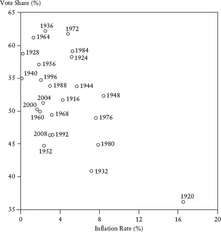
To see how the incumbent party vote share and inflation (or deflation) are related, Figure 1-2 graphs the vote share against inflation for the 24 elections between 1916 and 2008. According to the theory just discussed, there should be a negative relationship between the two: when inflation is high, the vote share should be low, and vice versa. You can see from Figure 1-2 that there does seem to be at least a slight negative relationship between the incumbent party vote share and inflation: the scatter of points has a slight downward pattern.

We are not, however, limited to a choice between one or the other—the growth rate or inflation. It may be that both the growth rate and inflation affect voting behavior. In other words, we need not assume that voters look at only one aspect of the economy when they are considering their future financial well-being. For example, if both the growth rate and inflation are high, a voter may be less inclined to vote for the incumbent party than if the growth rate is high and inflation is low. Similarly, if both the growth rate and inflation are low, a voter may be more inclined to vote for the incumbent party than if the growth rate is low and inflation is high.

FIGURE 1-2 Incumbent party vote share graphed against the inflation rate

An example of a high growth rate and low inflation is 1964, where the growth rate was about 5 percent and inflation was about 1 percent. In this case, the incumbent, President Johnson, won by a landslide over Barry Goldwater—receiving 61.2 percent of the two-party vote. An example of a low growth rate and high inflation is 1980, where the growth rate was about –4 percent and inflation about 8 percent. In this case, the incumbent, President Carter, lost by a large amount to Ronald Reagan—receiving only 44.8 percent of the two-party vote.

To carry on, we are also not limited to only two measures of the economy. In addition to observing how the economy has grown in the year of the election, voters may look at growth rates over the entire four years of the administration. In other words, past growth rates along with the growth rate in the election year may affect voting behavior. One measure of how good or bad past growth rates have been is the number of quarters during the four-year period of the administration in which the growth rate has exceeded some large number. These are quarters in which the output news was particularly good, and voters may be inclined to remember these kinds of events. There is some evidence from psychological experiments that people tend to remember peak stimuli more than they remember average stimuli, a finding that is consistent with voters remembering very strong growth quarters more than the others. Therefore, voters may be more inclined to vote for the incumbent party if there were many of these “good news quarters” during the administration than if there were few.

Noneconomic factors may also affect voting behavior. If the president is running for reelection, he (or maybe she in the future) may have a head start. He can perhaps use the power of the presidency to gain media attention, control events, and so forth. He is also presumably well known to voters, and so there may be less uncertainty in voters’ minds regarding the future if he is reelected rather than if someone new is elected. Voters who...

Table des matières

• Cover
• Copyright
• Title Page
• Contents
• Preface
• Introduction: What This Book Is About
• 1 It’s the Economy, Stupid
• 2 The Tools in Seven Easy Lessons
• 3 Presidential Elections
• 4 Congressional Elections
• 5 Extramarital Affairs
• 6 Wine Quality
• 7 College Grades and Class Attendance
• 8 Marathon Times
• 9 Aging and Baseball
• 10 Predicting College Football Games
• 11 Interest Rates
• 12 Inflation
• 13 More Things
• Chapter Notes
• Glossary
• Poetry Credits
• Index