Stochastic Drawdowns

Hongzhong Zhang

• Éditeur: WSPC
• Année: 2018
• ISBN:
  9789813141650
• Sujet: Mathematics
• Sous-sujet: Logic in Mathematics

-->

Stochastic Drawdowns consists of some recent advances on Dr Hongzhong Zhang's own quantitative research of the well-known risk measures, drawdowns and maximum drawdowns. In this book, the author provides an extensive probabilistic study of different aspects of drawdown risks, which include the drawdown risk in finite time-horizons, the speed of market crashes (drawdowns), the frequency of drawdowns, the occupation time (time in distress), and the duration of drawdowns. Leveraging the knowledge in stochastic calculus, Lévy processes and optimal stopping, these topics can be considered as problems in advanced applied stochastic processes, and insurance/financial mathematics.

The book also offers a number of applications of drawdowns in financial risk management, insurance, and algorithmic trading, including schemes on hedging and synthesizing of maximum drawdown options, (cancellable) drawdown insurance contracts and their fair premium, as well as optimal trading under drawdown-type constraints such as trailing stops.

It is the goal of this book to offer a comprehensive characterization of drawdown risks and a handful of applications of drawdown in practice. On the one hand, the book enables interested students and researchers to learn the state-of-art probabilistic research on drawdowns, and explore new mathematical problems that are of practical importance to the financial industry. On the other hand, the book provides financial practitioners with access to a variety of analytically tractable measurements of drawdown risks, and the insight into hedging, optimal trading and execution amid challenges of these risks.

--> Contents:

• Introduction
• Drawdown Measures:
  • Drawdowns Preceding Drawups in a Finite Time-Horizon
  • Drawdowns and the Speed of Market Crashes
  • Frequency of Drawdowns in a Brownian Motion Model
  • Occupation Times Related to Drawdowns
  • Duration of Drawdowns under Lévy Models
• Applications of Drawdown:
  • Maximum Drawdown Insurance Using Options
  • Fair Premiums of Drawdown Insurances
  • Optimal Trading with a Trailing Stop
• Appendix: Briefly on One-Dimensional Linear Diffusions

-->
--> Readership: Senior undergraduate and graduate students equipped with the knowledge of stochastic processes and financial practitioners who are interested in optimal trading and execution. -->
Keywords:Drawdown;Maximum Drawdown;Insurance;Optimal TradingReview: Key Features:

• The first book to touch on the advanced quantitative analysis of drawdowns in the current market
• A rigorous and extensive study of drawdowns from a probabilistic point of view
• Addressing of important practical problems related to drawdowns

Chapter 1

Introduction

Financial turmoils are most often marked with series of sharp falls in asset prices triggered by certain market events, with the recent examples of the S&P downgrade of US debt, and default speculations of European countries. Many individual and institutional investors are wary of large market drawdowns as they not only lead to portfolio losses and liquidity shocks, but also indicate potential imminent recessions. As is well known, hedge fund managers are typically compensated based on the fund’s outperformance over the last record maximum, or the high-water mark. As such, drawdown events can directly affect the manager’s income. Also, a major drawdown may also trigger a surge in fund redemption by investors, and lead to the manager’s job termination. Hence, fund managers have strong incentive to seek insurance against drawdowns (see, e.g., Burghardt et al. (2003)).

Formally, the drawdown is defined as the difference between the present value X_t of a portfolio or asset and its running maximum X_t := sup_s∈[0,t] X_s. That is,

Drawdowns provide a dynamic measure of risk in that they measure the drop of a stock price, index or value of a portfolio from its running maximum. They thus provide portfolio managers and commodity trading advisers a tool with which to assess the downside risk taken by a mutual fund during a given economic cycle. On the other hand, the maximum drawdown, which is defined as the running maximum of the drawdown process,

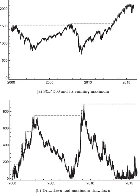
records the worst performance that could have happened in the past, and serves as an overall performance measure of the holding during a given period. To visualize the drawdown and the maximum drawdown processes, we illustrate in Figure 1.1 their sample paths for the S&P 500 index from January 3, 2000 to December 31, 2015.

Naturally, a prerequisite for controlling drawdown risks properly in practice is to understand them thoroughly. One popular probabilistic approach in study drawdowns is through probabilistic studies of the first passage time of the drawdown process, namely, for a given threshold a > 0, the stopping time defined as

Probabilistic characterizations of τ_D⁺(a) and other related quantities can provide investors information about drawdown risks from different angles. For instance, by {τ_D⁺(a) < T} = {D_T > a}, one gets the distribution of the maximum drawdown D_T from the distribution of τ_D⁺(a), and hence, the maximum drawdown or the downward momentum during an investment horizon can be assessed through relevant formulas for τ_D⁺(a); by studying excursions of the underlying process below its maximum until τ_D⁺(a), one obtains a measurement for the speed at which a large drawdown occurs.

On the other hand, protective means against a large drawdown of the underlying can be introduced by using the first passage time τ_D⁺(a) as the indicator for the drawdown events. For instance, a portfolio manager who suffers from the loss of income due to large positive realizations of maximum drawdown may be interested in a contract that pays the holder $1 at the maturity if the maximum drawdown exceeds a pre-specified level. Such a contract can be considered as a digital options that pays either one dollar or zero at the maturity T, depending on whether the event {τ_D⁺(a) < T} occurs or not.

Drawdown and its first passage time also play a meaningful role in trading practices to control/limit risks. In particular, a popular trade order called trailing stops, which is widely used by proprietary traders and retail investors to provide downside protection for an existing position, is to liquidate when the value of the existing position drops from its running maximum for more than a pre-specified percentage. While a trailing stop always limits the drawdown of the existing position capped, it is non-trivial to determine whether the investor can improve her expected payout from the trade by liquidating earlier. This motivates the investigation of the optimal liquidation prior a trailing stop, and optimal timing for setup the position with a trailing stop.

Fig. 1.1. (a) Plots of S&P 500 index (black) and its running maximum (gray dashed) from January 3, 2000 to December 31, 2015. (b) Plots of the drawdown process (black) and the maximum drawdown process (gray dashed) of S&P 500 index during the same period. These plots reveal that the market has experienced two major cycles in this period. Moreover, while it took about 7.5 years for the market to fully recover in the first cycle, it only took 5.5 years in the second cycle.

In this book, we take the aforementioned first passage time approach to study drawdowns and address some practically important applications of drawdowns in financial engineering. Specifically, in Part I of the book, we study probabilistic properties of drawdowns in five aspects, namely, the finite time-horizon property, the speed, the frequency, the occupation times, and the durations, of drawdowns. Through Laplace transforms, we provide rigorous mathematical analysis and calculations for these quantities under diffusion models and Lévy models. In Part II of the book, we focus on applications in drawdowns, including replication of maximum drawdown options, fair evaluation of drawdown insurances, and optimal trading with a trailing stop. The objective of the book is to offer both researchers from academia and practitioners an overview of the state-of-art probabilistic research on drawdowns and a better understanding of the hedging and optimal trading amid challenges arise from drawdown risks.

1.1.Chapter Outline

We begin our journey to the subject of drawdown in Chapter 2, where we determine the probability that a drawdown of a units precedes a drawup of b units in a finite time-horizon. Formally, the drawup of a stochastic process X_⋅ is defined as

where X_t := inf_s∈[0,t] X_s denotes the running minimum of X_⋅. Thus, this probability assesses the relative strength of downside risk (drawdown) compared to upward momentum (drawup) over a finite time-horizon. To determine this probability, we first consider the simple case with equal-sized drawdown/drawup (i.e., a = b), and derive analytic formulas of this probability by drawing connections to the first exit problems under a simple random walk model and a Brownian motion with drift model. For the general case, we randomize the time-horizon with an independent exponential random variable — a technique known as Canadization, and reduce the probability of interest to the Laplace transform of the first passage time of the drawdown when it precedes a drawup. Using a classical approximation argument as in Lehoczky (1977), we derive analytical formulas for this Laplace transform under general linear diffusion models. Finally, we use Laplace inversion to evaluate the drawdown preceding drawup probability and the conditional density of the maximum relative drawup given a drawdown event, under a geometric Brownian motion (GBM) model.

Apart from the finite time-horizon properties of drawdowns and drawups, the issue of how fast a market crash occurred is also of vital importance to investors and portfolio or hedge fund managers. This motivates us to study the joint distribution of the drawdown and the speed at which it is realized in Chapter 3. In particular, we measure the speed of market crash by the time elapsed between the first passage time of the drawdown to level a > 0, τ_D⁺(a), and the last reset time of the running maximum prior to that drawdown, g_a := sup{t < ...

Table des matières

• Cover
• Halftitle
• Series Editors
• Title
• Copyright
• Dedication
• Preface
• Contents
• About the Author
• 1. Introduction
• Part I Drawdown Measures
• Part II Applications of Drawdown
• Appendix. Briefly on One-Dimensional Linear Diffusions
• Bibliography
• Index