Bayesian Inference in the Social Sciences

Ivan Jeliazkov, Xin-She Yang, Ivan Jeliazkov, Xin-She Yang

• Éditeur: Wiley
• Année: 2014
• ISBN:
  9781118771129
• Édition: 1
• Sujet: Mathematics
• Sous-sujet: Probability & Statistics

Presents new models, methods, and techniques and considers important real-world applications in political science, sociology, economics, marketing, and finance Emphasizing interdisciplinary coverage, Bayesian Inference in the Social Sciences builds upon the recent growth in Bayesian methodology and examines an array of topics in model formulation, estimation, and applications. The book presents recent and trending developments in a diverse, yet closely integrated, set of research topics within the social sciences and facilitates the transmission of new ideas and methodology across disciplines while maintaining manageability, coherence, and a clear focus. Bayesian Inference in the Social Sciences features innovative methodology and novel applications in addition to new theoretical developments and modeling approaches, including the formulation and analysis of models with partial observability, sample selection, and incomplete data. Additional areas of inquiry include a Bayesian derivation of empirical likelihood and method of moment estimators, and the analysis of treatment effect models with endogeneity. The book emphasizes practical implementation, reviews and extends estimation algorithms, and examines innovative applications in a multitude of fields. Time series techniques and algorithms are discussed for stochastic volatility, dynamic factor, and time-varying parameter models. Additional features include:

• Real-world applications and case studies that highlight asset pricing under fat-tailed distributions, price indifference modeling and market segmentation, analysis of dynamic networks, ethnic minorities and civil war, school choice effects, and business cycles and macroeconomic performance
• State-of-the-art computational tools and Markov chain Monte Carlo algorithms with related materials available via the book's supplemental website
• Interdisciplinary coverage from well-known international scholars and practitioners

Bayesian Inference in the Social Sciences is an ideal reference for researchers in economics, political science, sociology, and business as well as an excellent resource for academic, government, and regulation agencies. The book is also useful for graduate-level courses in applied econometrics, statistics, mathematical modeling and simulation, numerical methods, computational analysis, and the social sciences.

CHAPTER 1

BAYESIAN ANALYSIS OF DYNAMIC NETWORK REGRESSION WITH JOINT EDGE/VERTEX DYNAMICS

ZACK W. ALMQUIST¹ AND CARTER T. BUTTS²

¹University of Minnesota, USA.

²University of California, Irvine, USA.

1.1 Introduction

Change in network structure and composition has been a topic of extensive theoretical and methodological interest over the last two decades; however, the effects of endogenous group change on interaction dynamics within the context of social networks is a surprisingly understudied area. Network dynamics may be viewed as a process of change in the edge structure of a network, in the vertex set on which edges are defined, or in both simultaneously. Recently, Almquist and Butts (2014) introduced a simple family of models for network panel data with vertex dynamics—referred to here as dynamic network logistic regression (DNR)—expanding on a subfamily of temporal exponential-family random graph models (TERGM) (see Robins and Pattison, 2001; Hanneke et al., 2010). Here, we further elaborate this existing approach by exploring Bayesian methods for parameter estimation and model assessment. We propose and implement techniques for Bayesian inference via both maximum a posteriori probability (MAP) and Markov chain Monte Carlo (MCMC) under several different priors, with an emphasis on minimally informative priors that can be employed in a range of empirical settings. These different approaches are compared in terms of model fit and predictive model assessment using several reference data sets.

This chapter is laid out as follows: (1) We introduce the standard (exponential family) framework for modeling static social network data, including both MLE and Bayesian estimation methodology; (2) we introduce network panel data models, discussing both MLE and Bayesian estimation procedures; (3) we introduce a subfamily of the more general panel data models (dynamic network logistic regression)—which allows for vertex dynamics—and expand standard MLE procedures to include Bayesian estimation; (4) through simulation and empirical examples we explore the effect of different prior specifications on both parameter estimation/hypothesis tests and predictive adequacy; (5) finally, we conclude with a summary and discussion of our findings.

1.2 Statistical Models for Social Network Data

The literature on statistical models for network analysis has grown substantially over the last two decades (for a brief review see Butts, 2008b). Further, the literature on dynamic networks has expanded extensively in this last decade – a good overview can be found in Almquist and Butts (2014). In this chapter we use a combination of commonly used statistical and graph theoretic notation. First, we briefly introduce necessary notation and literature for the current state of the art in network panel data models, then we review these panel data models in their general form, including their Bayesian representation. Last, we discuss a specific model family (DNR) which reduces to an easily employed regression-like structure, and formalize it to the Bayesian context.

1.2.1 Network Data and Nomenclature

For purposes of this chapter, we will focus on networks (social or otherwise) that can be represented in terms of dichotomous (i.e., unvalued) ties among pairs of discrete entities. [For more general discussion of network representation, see, e.g., Wasserman and Faust (1994); Butts (2009).] We represent the set of potentially interacting entities via a vertex set (V), with the set of interacting pairs (or ordered pairs, for directed relationships) represented by an edge set (E). In combination, these two sets are referred to as a graph, G = (V, E). (Here, we will use the term “graph” generically to refer to either directed or undirected structures, except as indicated otherwise.) Networks may be static, e.g., representing relationships at a single time point or aggregated over a period of time, or dynamic, e.g., representing relationships appearing and disappearing in continuous time or relationship status at particular discrete intervals.

For many purposes, it is useful to represent a graph in terms of its adjacency matrix: for a graph G of order N = |V|, the adjacency matrix Y

{0, 1}^{N × N} is a matrix of indicator variables such that Y_ij = 1 iff the ith vertex of G is adjacent (i.e., sends a tie to) the jth vertex of G. Following convention in the social network (but not graph theoretic) literature, we will refer to N as the size of G.

The above extends naturally to the case of dynamic networks in discrete time. Let us consider the time series …, G_t−1, G_t, G_t+1,…, where G_t = (V_t, E_t) represents the state of a system of interest at time t. This corresponds in turn to the adjacency matrix series …, Y_..t−1, Y_..t, Y_..t+1,…, with N_t = |V_t| being the size of the network at time t and Y_..t

{0, 1}^N_txN_t such that Y_ijt = 1 iff the ith vertex of G_t is adjacent to the jth vertex of G_t at time t. As this notation implies, the vertex set of an evolving network is not necessarily fixed; we shall be particularly interested here in the case in which V_t is drawn from some larger risk set, such that vertices may enter and leave the network over time.

1.2.2 Exponential Family Random Graph Models

When modeling social or other networks, it is often helpful to represent their distributions via random graphs in discrete exponential family form. Graph distributions expressed in this way are called exponential family random graph models or ERGMs. Holland and Leinhardt (1981) are generally credited with the first explicit use of statistical exponential families to represent random graph models for social networks, with important extensions by Frank and Strauss (1986) and subsequent elaboration by Wasserman and Pattison (1996), Pattison and Wasserman (1999), Pattison and Robins (2002), Snijders et al. (2006), Butts (2007), and others. The power of this framework lies in the extensive body of inferential, computational, and stochastic process theory [borrowed from the general theory of discrete exponential families, see, e.g., Barndorff-Nielsen (1978); Brown (1986)] that can be brought to bear on models specified in its terms.

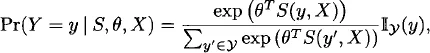
We begin with the “static” case in which we have a single random graph, G, with support G. It is convenient to model G via its adjacency matrix Y, with y representing the associated support (i.e., the set of adjacency matrices corresponding to all elements in G). In ERGM form, we express the pmf of Y as follows:

(1.1)

where

is a vector of sufficient statistics, θ

^s is a vector of natural parameters, X

X is a collection of covariates, and

_y is the indicator function (i.e., 1 if its argument is in the support of y, 0 otherwise).¹ If |G| is finite, then the pmf for any G can obviously be written with finite-dimensional S, θ (e.g., by letting S be a vector of indicator variables for elements of y); this is not necessarily true in the more general case, although a representation with S, θ of countable dimension still exists. In practice, it is generally assumed that S is of low dimension, or that at least that the vector of natural parameters can be mapped to a low-dimensional vector of “curved” parameters [see, e.g., Hunter and Handcock (2006)].

While the extreme generality of this framework has made it attractive, model selection and parameter estimation are often difficult due to the normalizing factor (κ(θ, S, X) = ∑y′

y exp(θ^T S(y′, X))) in the denominator of equation (1.1). This normalizing factor is analytically intractable and difficult to compute, except in special cases such as the Bernoulli and dyad-multinomial random graph families (Holland and Leinhardt, 1981); the first applications of this family (stemming from Holland and Leinhardt’s seminal 1981 paper) focused on these special cases. Later, Frank and Strauss (1986) introduced a more general estimation procedure based on cumulant methods, but this proved too unstable for practical use. This, in turn, led to an emphasis on approximate inference using maximum pseudo-likelihood (MPLE) estimation (Besag, 1974), as popularized in this application by Strauss and Ikeda (1990) and later Wasserman and Pattison (1996). Although MPLE coincides with maximum likelihood estimation (MLE) in the limiting case of edgewise independence, the former was found to be a poor approximation to the MLE in many practical settings, thus leading to a consensus against its general use [see, e.g., Besag (2001) and van Duijn et al. (2009)]. The late 1990s saw the development of effective Markov chain Monte Carlo strategies for simulating draws from ERG models (Anderson et al., 1999; Snijders, 2002) which led to the current focus on MLE methods based either on first order method of moments (which coincides with MLE for regular ERGMs) or on importance sampling (Geyer and Thompson, 1992).²

Theoretical developments in the ERGM literature have arguably lagged inferential and computational advances, although this has become an increasingly active area of research. A major concern of the theoretical literature on ERGMs is the problem of degeneracy, defined differently by different authors but generally involving an inappropriately large concentration of probability mass on a small set of (generally unrealistic) structures. This issue was recognized as early as Strauss (1986), who showed asymptotic concentration of probability mass on graphs of high density for models based on triangle statistics. [This motivated the use of local triangulation by Strauss and Ikeda (1990), a recommendation that went unheeded in later work.] More general treatments of the degeneracy problem can be found in Handcock (2003), Schweinberger (2011), and Chatterjee and Diaconis (2011). Butts (2011) introduced analytical methods that can be used to bound the behavior of general ERGMs by Bernoulli graphs (i.e., ERGMs with independent edge variables), and used these to show sufficient conditions for ERGMs to avoid certain forms of degeneracy as N → ∞. One area of relatively rich theoretical development in the ERGM literature has been the derivation of sufficient statistics from first pr...

Table des matières

• Cover
• Half Title page
• Title page
• Copyright page
• Preface
• Chapter 1: Bayesian Analysis of Dynamic Network Regression with Joint Edge/Vertex Dynamics
• Chapter 2: Ethnic Minority Rule and Civil War: A Bayesian Dynamic Multilevel Analysis
• Chapter 3: Bayesian Analysis of Treatment Effect Models
• Chapter 4: Bayesian Analysis of Sample Selection Models
• Chapter 5: Modern Bayesian Factor Analysis
• Chapter 6: Estimation of Stochastic Volatility Models with Heavy Tails and Serial Dependence
• Chapter 7: From the Great Depression to the Great Recession: A Model-Based Ranking of U.S. Recessions
• Chapter 8: What Difference Fat Tails Make: A Bayesian MCMC Estimation of Empirical Asset Pricing Models
• Chapter 9: Stochastic Search for Price Insensitive Consumers
• Chapter 10: Hierarchical Modeling of Choice Concentration of U.S. Households
• Chapter 11: Approximate Bayesian Inference in Models Defined Through Estimating Equations
• Chapter 12: Reacting to Surprising Seemingly Inappropriate Results
• Chapter 13: Identification and MCMC Estimation of Bivariate Probit Models with Partial Observability
• Chapter 14: School Choice Effects in Tokyo Metropolitan Area: A Bayesian Spatial Quantile Regression Approach
• Index