Logistic Population Growth

11 Key excerpts on "Logistic Population Growth"

• 

  eBook - PDF

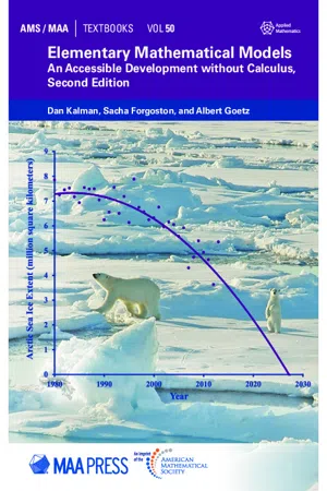
  Elementary Mathematical Models

  An Accessible Development without Calculus, Second Edition

  • Dan Kalman, Sacha Forgoston, Albert Goetz(Authors)
  • 2019(Publication Date)
  • American Mathematical Society

    (Publisher)

  364 Chapter 6. Logistic Growth to grow, the rate of growth tapers off. Each year the percentage of increase is less than for the preceding year. Eventually, the population starts to level off near 50,000 . If you examine the data carefully, you will see that the population actually goes a little above 50,000 . Then it jumps back and forth. One year it is a little less than 50,000 , the next it is a little more, then a little less, then a little more. The population size continues to fluctuate back and forth, all the while edging closer to the 50,000 figure. Remember that we picked 50,000 as the size at which the population would remain fixed from year to year. This introductory discussion shows how a simple model can be modified to ob-tain more realistic behavior. Earlier models with geometric growth assumed that the growth factor would remain constant no matter what the population size. In this pre-sentation we built up a new model that includes variation in the growth factor. Ad-mittedly, using a linear model for this variation imposes its own limitations. But the resulting model is much more realistic than simple geometric growth. In a true appli-cation, we might next try to measure the way the growth factor actually varies as the population grows, and fit the best linear model possible to the data. That would give us a logistic growth model that could be tested for accuracy in the real world. As a matter of fact, logistic models often appear in applications, and not just for growth of biological populations. Another example of limited growth is provided by sales of new consumer electronics devices, such as cell phones. Initially, sales increase rapidly, but new sales decline as the market becomes saturated. That is another context for which a logistic model might be adopted. At the end of this section we will see an example of fitting a logistic growth sequence to actual data. But now we turn to an investigation of the properties of logistic growth sequences.

  Sign up to read

  Learn more about book
• 

  eBook - PDF

  Population Dynamics

  Alternative Models

  • Bertram G. Jr. Murray(Author)
  • 2013(Publication Date)
  • Academic Press

    (Publisher)

  The logistic equation has been criticized frequently (Gray, 1929; Hog-ben, 1931; Kavanagh and Richards, 1934; Feller, 1940; Andrewartha and Birch, 1954; Smith, 1952, 1954; Pielou, 1969, 1977), mainly because more than one equation can fit the same data set, and each equation has different biological properties. Furthermore, population growth of animals 20 2: POPULATION MATHEMATICS with complex life histories does not often conform to the logistic (An-drewartha and Birch, 1954). The advantages of the logistic are its simplic-ity, compared with alternatives, and its reality, meaning that its con-stants have biological meaning (Andrewartha and Birch, 1954). The logistic is also attractive because its density-dependent growth rate is consistent with the logical notion of density-dependent regulation (Lack, 1966), al-though, it should be noted, at least one promoter of density dependence explicitly rejected the logistic equation as a model of population growth (Nicholson, 1958b). The logistic model, as any model, has limitations. Pielou (1969, 1977) listed the restrictive assumptions, which must frequently be false: (1) The abiotic environment is sufficiently constant that birth and death rates are unaffected; (2) crowding affects all individuals of the population equally; (3) birth and death rates respond instantly to changes in density; (4) the population's growth rate is density-dependent even at low densities; (5) the population maintains a stable age distribution; and (6) the females in sexually reproducing populations always find mates. Pielou (1969, 1977) mentions that if assumptions (4) and (6) were incorrect, the effects would cancel each other. But even so, assumptions (3) and (5) are incompatible. Any change in the age-specific death rates changes the stable age distribu-tion (see next section). Thus, under no circumstances can these six as-sumptions be exhibited by a population.

  Sign up to read

  Learn more about book
• 

  eBook - PDF

  Modelling and Quantitative Methods in Fisheries

  • Malcolm Haddon(Author)
  • 2011(Publication Date)
  • Chapman and Hall/CRC

    (Publisher)

  It has also been suggested that at least part of the sad history of failures in fishery advice and management stems from this combination (Larkin, 1977); this suggestion is often followed by implied abuse at the logis-tic and its implications, as well as the people who use it. However, invective against the logistic is misplaced. The logistic is simply a convenient model of linear density-dependent effects (similar fisheries advice would have come from any equilibrium analysis using a linear model of population regula-tion). Beverton and Holt (1957) pointed out the weaknesses inherent in using the Logistic Population Growth curve, but they recognized that in the absence of detailed information this approach might still have value if used carefully. They stated: It is when such detailed information does not exist that the sigmoid curve theory, by making the simplest reasonable assumption about the dynamics of a population, is valuable as a means of obtaining a rough appreciation from the minimum of data. (Beverton and Holt, 1957, p. 330) The exponential population growth model was density independent in its dynamics; that is, the birth and death rates were unaffected by the population 26 Modelling and Quantitative Methods in Fisheries © 2011 by Taylor & Francis Group, LLC size. If population growth was regulated such that the difference between births and deaths was not a constant but became smaller as population size increased and greater as the population decreased, then the likelihood of runaway population growth or rapid extinction could be greatly reduced. Such a modification of the dynamic response with respect to density is what makes such models density dependent. In a density-dependent model, the population rate of increase (as a balance between births and deaths) alters in response to population size changes (Figure 2.2).

  Sign up to read

  Learn more about book
• 

  eBook - PDF

  Introduction to Population Biology

  • Dick Neal(Author)
  • 2018(Publication Date)
  • Cambridge University Press

    (Publisher)

  The issue of estimating the carrying capacity and rate of increase for populations that have already been harvested is also considered. The strategy can be extremely risky. The carrying capacity may fluctuate, and estimations of K and r m are not without error; in addition, any errors accumulate so that MSY estimates may not be reliable (see Simulations website). Populations need to be monitored very carefully, and if the carrying capacity is variable, it is very easy to overfish (i.e. drive the population below K/2). Obviously, one should immediately reduce the harvest, but there are often political pressures to delay doing this. Once a fishery has collapsed, its recovery is by no means assured, even if the fishing levels are reduced to zero. 66 Logistic Growth 5.7 Summary and Conclusions The logistic growth curve is one mathematical model that describes Darwin’ s ‘struggle for existence’ when the struggle involves only intraspecific competition for resources. The model assumes that the population consists of identical individuals that are growing in a constant environment of defined limits or size. As the population increases, intraspecific competition for resources also increases, and the individuals adjust their growth rates accordingly as they utilize the fixed resources of the environment. The model describes an S-shaped form of growth to a stable carrying capacity, K, which depends on the characteristics of the population and the number of resources available in the environment, while the steepness of the curve depends on the per capita rate of increase, r . The restrictive assumptions of the model may be relaxed to analyse how factors such as time lags and a variable environment affect the form of population growth. These analyses show that time lags have surprisingly little effect on the form of population growth for populations with low r values.

  Sign up to read

  Learn more about book
• 

  eBook - PDF

  Animal Population Ecology

  An Analytical Approach

  • T. Royama(Author)
  • 2021(Publication Date)
  • Cambridge University Press

    (Publisher)

  The article was ‘On the logistic law of growth and its empirical verifications in biology’ (Feller, 1940). In it, the author pointed out that it was a law without a theory and that it would be dangerous to rely solely on empirical verifications. Pat gave it to me, hinting that I might think about a possible theory. Although I kept the idea in mind, I shelved it for several years. One day, I was playing with dots and circles on a sheet of graph paper to figure out a problem about the geometry of a predator searching for prey. Suddenly a thought struck and I ‘slapped my lap’, a Japanese expression for an ‘aha!’ moment. For the next few weeks, I concentrated on the subject and managed to derive the logistic equation from the ecological principle of intraspecific (within-population) competition, originally published in Royama (1992, section 4.2.5). Since then, the theory I conceived has become a fundamental basis of my ecological studies of populations that I talk about in this book. In the following, I begin with a short history of the development of the classical logistic model. 3.2 The Classical Logistic Equation Back in mid-nineteenth-century Belgium, the mathematician Pierre- François Verhulst, inspired by his mentor Adolphe Quetelet during a discussion on socioeconomic issues, began to work on the problem of the then influential idea of the Malthusian geometric progression of popula- tions. [Thomas Robert Malthus was the English cleric and the author of the well-known (1798) treatise ‘An Essay on the Principle of Population’.] The Malthusian theory (as it is popularly known) is essen- tially this: a human population grows at a rate of geometric progression, whereas essential resources (food supplies) grow only at a rate of arith- metic progression. Therefore, unless the population was controlled by some social or moral disciplines, only catastrophes like epidemics, famines, or wars could reduce the population to a level at which the resources could sustain it.

  Sign up to read

  Learn more about book
• 

  eBook - PDF

  Mathematical Modeling in the Social and Life Sciences

  • Michael Olinick(Author)
  • 2014(Publication Date)
  • Wiley

    (Publisher)

  The environment has a carrying capacity, an upper limit on the number of individual organisms that can exist on the available resources. As the size of the population gets closer to this carrying capacity, its rate of growth must slow down. Any realistic model of population dynamics should reflect this feature. This section examines a mathematical model that attempts to do this. Briefly stated, the argument in the paragraph above is that the rate of growth is not constant, but rather is dependent on the size of the population. The mathematical model should then assert that the rate of population is in fact a function of the population; mathematically, the statement looks like dP dt = f P 17 where f is some function of population size P. How should f be selected? If the population ever reaches a zero level, then of course it will always remain at zero. Hence, the function f 72 CHAPTER 3 Ecological Models: Single Species should have the property that f 0 = 0. Suppose we write the function f as f P = Pg P where g is also a function of P. Then f 0 = 0g 0 = 0 regardless of the form of the function g. Note that we can think of g as the per capita growth rate, g P = P P. How then should g be selected? The idea that rate of growth will slow down as population gets larger and larger can be captured by the condition that g′ P be negative. The simplest model is then obtained by making the function g as simple as possible—namely, assume that g is a linear function, g P = a − bP 18 where a and b are positive constants. Then the model assumes the form dP dt = P a − bP 19 This assertion is called the logistic equation or the Verhulst-Pearl equation. Note that this derivation of the logistic model does not make explicit use of the carrying capacity of the environment. There are several other ways of arriving at this model. We will outline one path: suppose that aP is the rate at which the population would increase if the environment possessed unlimited space and resources.

  Sign up to read

  Learn more about book
• 

  eBook - PDF

  Dynamical Systems for Biological Modeling

  An Introduction

  • Fred Brauer, Christopher Kribs(Authors)
  • 2015(Publication Date)
  • Chapman and Hall/CRC

    (Publisher)

  However, as the populations reached their carrying capacities, they exhibited ongoing, significant fluctuations, gaining or losing over 25% in a handful of years (see Figures 3.6 and 3.7). Davidson’s work is not the only instance where a logistic model fits data well only during the initial rapid growth period. Renshaw discusses (e.g., p. 55) several other situations in which lab cultures and other populations were observed to grow more or less logistically toward carrying capacity, but there-after exhibited either sustained fluctuations or a gradual decline. The likely explanation for this phenomenon is that when a population has not yet run up against resource limitations, its reproductive capacity may often be the strongest force affecting its growth, whereas other factors such as stochastic effects, spatial heterogeneity, or changes in the environment (the fluctuations observed in the Australian sheep populations in the graphs were attributed to fluctuations in carrying capacity while pastures recovered from overgrazing) dominate when the logistic growth is small. In any case, the conclusion to draw 11 J. Davidson, On the ecology of the growth of the sheep population in South Australia, Transactions of the Royal Society of South Australia 62: 141–148, 1938. J. Davidson, On the growth of the sheep population in Tasmania, Transactions of the Royal Society of South Australia 62: 342–346, 1938. 114 Dynamical Systems for Biological Modeling: An Introduction 1860 1880 1900 1920 1940 year 2000 4000 6000 8000 kilosheep FIGURE 3.6 : South Australian sheep population (in thousands) from 1838 to 1936 with the logistic curve y ( t ) = 7115 / [1 + exp(249 . 11 − 0 . 13369 t )] superimposed, after Ren-shaw (1995). 1840 1860 1880 1900 1920 year 500 1000 1500 2000 kilosheep FIGURE 3.7 : Tasmanian sheep population (in thousands) from 1818 to 1936 with the logistic curve y ( t ) = 1670 / [1 + exp(240 . 81 − 0 . 13125 t )] su-perimposed, after Renshaw (1995).

  Sign up to read

  Learn more about book
• 

  eBook - PDF

  Mathematical Modelling of Environmental and Ecological Systems

  • J.B. Shukla, T.G. Hallam, V. Capasso(Authors)
  • 2012(Publication Date)
  • Elsevier Science

    (Publisher)

  5 SUMMARY In this paper, economic growth models with logistic population and technology have been investigated in the cases of plentiful resources (no scarce resource) and exhaustible resources. By a suitable choice of labour-population relation the dynamics of the out-put capital ratio and rate of resource utilization have been investigated. In the case of a plentiful resource, it has been noted that the positive equilibrium point does not depend upon the intrinsic growth rate no when population and technology follow logistic behaviour. It has been established that the economy may follow a sustainable path for a wide range of economic parameters (see condition (16)). In the case of an exhaustible resource, it has been concluded that under appropriate conditions the economy which in other situations may be unstable, may follow a stable growth path. 6 REFERENCES Arrow, K.J., (1962). The Economic Implications of Learning by Doing. Rev. of Eco. Studies, 29:155-173. Cigno, A., (1981). Growth with Exhaustible Resources and Endogeneous Populations. Rev. of Eco. Studies 43: 281-287. , (1984a). Further Implications of Learning by Doing. Bull, of Eco. Res. 36: 97-108. , (1984b). Consumption vs. Procreation in Economic Growth. In Economic Consequences of Population Change in Industrialised Countries. Edited by G. Steinmann, Springer-Verlag, Berlin. Gompertz, B., 1825. On the Nature of the Function Expressive of the Law of Human Mortality, and on a New Method of Determining the Values of Life Contingencies. Philo. Trans, of Royal. Soc. 36: 513-585. Kelley, A.C., 1974. The Role of Population in Models of Economic Growth. Amer. Eco. Rev. 64: 39-44. Kosobud, R.F., and O'Neill, W.D., 1974. A Growth Model with Population Endogeneous. Amer. Eco. Rev. 44: 27-34. LaSalle, J.P. and Lefschetz, S., 1961. Stability by Liapunov's Direct Method and Applications. Academic Press, New York. Laitner, J., 1984. Resource Extraction Costs and Competitive Steady-State Growth.

  Sign up to read

  Learn more about book
• 

  eBook - PDF

  Population Ecology

  An Introduction to Computer Simulations

  • Ruth Bernstein(Author)
  • 2003(Publication Date)
  • Wiley

    (Publisher)

  44n1=logistic(3,100,1,101,25); 44n2=logistic(3,100,1,99,25); 44figure 44hold on Graph the population densities as a function of time with 44plot(0:25,n1(1:26), ’r’) 44plot(0:25,n2(1:26), ’b’) Label the graph, transfer it to a Word document, and write a ¢gure legend. Explain why populations with high maximum rates of growth should not be used in controlled experiments. This graph also shows another feature of chaos: initial conditions (here, initial densities) can generate very di¡erent outcomes. Logistic Population Growth: DiscreteTime Model 45 EXERCISE 7 Interspeci¢c Competition and Coexistence Interspeci¢c competition is competition between two species for a resource that is limited in supply. The classic model was developed by V|to Volterra, an Italian mathe- matician, in 1926. Later, in 1932, Alfred Lotka, an American population biologist, developed a way of analyzing the model in graphical form. The model consists of the di¡erental equation for Logistic Population Growth (continuous time) plus a term that describes the negative e¡ect of one species on the other. Here, we will develop the competition equations from the theta version of the logistic equation, because it is more versatile than the classic logistic equation. dN dt ¼ r m N  1   N K  y  ð7:1Þ The equation for the growth of species 1 when it experiences competition from species 2 is written dN 1 dt ¼ r mð1Þ N 1  1   N 1 K 1  y 1  a 12 N 2 K 1  ð7:2Þ where r mð1Þ is the maximum rate of growth per individual for species 1, a 12 is the e¡ect of an individual of species 2 on an individual of species 1 as compared with the e¡ect of an individual for species 1 on another individual of species 1 (de¢ned as being equal to 1). Population Ecology: An Introduction to Computer Simulations. By Ruth Bernstein. & 2003 John W|ley & Sons, Ltd

  Sign up to read

  Learn more about book
• 

  eBook - PDF

  Models for Ecological Data

  An Introduction

  • James S. Clark(Author)
  • 2020(Publication Date)
  • Princeton University Press

    (Publisher)

  (2003). These references are highly recommended for ecologists who study populations, as they contain more analysis of models than is included here. I provide a condensed treatment of this material, but empha- size aspects of models that will be important as we begin to incorporate data in Part II. For ecologists who do not study population-level phenomena, I recom- mend this section for general background on model development. 2.1 A Model and Data Example In the early part of this century Raymond Pearl (1925) used a simple sigmoid (logistic) curve, which he sometimes referred to as the law of population growth, to predict that the U.S. population would reach an upper limit of 197 million shortly after the year AD 2000 (Figure 2.1a) (Pearl 1925; Kingsland 1985). The basis for this prediction was U.S. Census Bureau data, from which he obtained decadal population statistics from AD 1790 to 1910, and the model in which he placed great faith—so much faith that he reported the inflection point of the curve to lie at April Fools Day, AD 1914. Note from Figure 2.1a that pop- ulation sizes after 1910 are based on extrapolation. The future has come to pass, and the modern census data do not look like the predictions of the early twentieth century (Figure 2.1b). History provides two lessons that this and subsequent chapters explore: (1) models can be importantly wrong (they may fit well for the wrong reasons), and (2) model evaluation requires estimates of uncertainty. CHAPTER 2 a) Pearl's law b) Through AD 2000 r = 0.0278 K = 326 1800 1850 1900 1950 2000 1800 1850 1900 1950 2000 AD year c) "Density effect" on population growth CD Q. O jf §•=§. a. CO 6 .20 Fitted through 2000 census Fitted through 1910 census 100 Millions 200 FIGURE 2.1. (a) Pearl's logistic curve fitted to U.S. Census Bureau data from 1790 through 1910. (b) A comparison with the longer series available in AD 2000.

  Sign up to read

  Learn more about book
• 

  eBook - ePub

  Understanding Nature

  Ecology for a New Generation

  • Louise M. Weber(Author)
  • 2023(Publication Date)
  • CRC Press

    (Publisher)

  Chapter 17 . In brief, the neutral theory approaches any ecological situation with the premise of no equilibrium, then determines if the accompanying data show otherwise. This approach applies to all ecological interactions, not just population growth. For instance, instead of assuming that predators and prey affect one another because that is what past theory suggests, the neutralists advocate an expectation of no interaction, then make a determination based on whether this hypothesis is violated. Interestingly, equilibrium states have been found for populations, but in small patches for short periods. Biotic processes as hypothesized by the equilibrists may indeed be at work as predicted, but in a constantly shifting mosaic of small patches.

  The equilibrium debate in population ecology diminished in the 1980s as practitioners began to turn toward conservation biology, the growth of rare species, and other practical applications. The equilibrium debate, however, migrated to community ecology, where it became an argument about interspecific interactions. Chapter 17 further describes this development of the equilibrium debate.

  THINKING QUESTIONS

  1. Why is the model named “logistic?” Use the internet to find out.
  2. Find examples of population growth for other species.Data from Christmas Bird Counts are available via internet.How might data for bird species collected during annual Audubon Club counts be somewhat biased?
  3. For the examples in this chapter that show boom and bust or erratic growth patterns,such as Red-breasted Nuthatch,examine the diet,life histories,and habitat requirements to speculate on the immediate causes of variation from year to year.
  4. How can chance,randomness,patchiness,perhaps even chaos be responsible for patterns we see in nature like the formation of biomes?
  5. Mayflies have an adult emergence period of only a few days (earning the apt name Order Ephemeroptera).So many adults swarm at once that snowplow equipment has been used to remove piles of cast juvenile skins and dead adults from the streets of waterfront towns.Likewise,17-year cicada adults can be so numerous that dogs and other animals get sick from eating too many. Describe situations like this you have experienced.Does heavy predation on cicadas still leave enough adults to lay eggs and renew the cycle?
  6. Fox (2011 ) has relegated the r and K selected species idea to the list of Zombie Ideas in Ecology – ideas now hard to kill.Widely believed and intuitively appealing,they tend to persist,according to Fox,in spite of repeated theoretical refutations and whole piles of contrary facts. In his words,they are undead.As a solution,Read and Harvey (1989

  Sign up to read

  Learn more about book