Parametric Parabolas

8 Key excerpts on "Parametric Parabolas"

• 

  eBook - PDF

  Calculus

  Single Variable

  • Howard Anton, Irl C. Bivens, Stephen Davis(Authors)
  • 2022(Publication Date)
  • Wiley

    (Publisher)

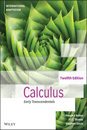
  588 CHAPTER 10 windujedi/iStockphoto Mathematical curves, such as the spirals in the center of a sunflower, can be described conveniently using ideas developed in this chapter. Parametric and Polar Curves; Conic Sections In this chapter we will study alternative ways of expressing curves in the plane. We will begin by studying parametric curves: curves described in terms of component functions. This study will include methods for finding tangent lines to parametric curves. We will then introduce polar coordinate systems and discuss methods for finding tangent lines to polar curves, arc length of polar curves, and areas enclosed by polar curves. Our attention will then turn to a review of the basic properties of conic sections: parabolas, ellipses, and hyperbolas. Finally, we will consider conic sections in the context of polar coordinates and discuss some applications in astronomy. 10.1 Parametric Equations; Tangent Lines and Arc Length for Parametric Curves Graphs of functions must pass the vertical line test, a limitation that excludes curves with self- intersections or even such basic curves as circles. In this section we will study an alternative method for describing curves algebraically that is not subject to the severe restriction of the ver- tical line test. We will then derive formulas required to find slopes, tangent lines, and arc lengths of these parametric curves. We will conclude with an investigation of a classic parametric curve known as the cycloid. Parametric Equations Suppose that a particle moves along a curve C in the xy-plane in such a way that its x- and y-coordinates, as functions of time, are x = f (t), y = g(t) We call these the parametric equations of motion for the particle and refer to C as the trajectory of the particle or the graph of the equations (Figure 10.1.1). The variable t is called the parameter x y C (x, y) A moving particle with trajectory C FIGURE 10.1.1 for the equations.

  Sign up to read

  Learn more about book
• 

  eBook - ePub

  Geometry for Naval Architects

  • Adrian Biran(Author)
  • 2018(Publication Date)
  • Butterworth-Heinemann

    (Publisher)

  Chapter 4

  Parametric Curves

  Abstract

  A curve can be represented by an implicit equation,

  f ( x , y ) = 0

  ,

  f ( x , y , z ) = 0

  , by an explicit equation,

  y = f ( x )

  ,

  z = f ( x , y )

  , or by parametric equations,

  x =

  f 1

  ( t )

  ,

  y =

  f 2

  ( t )

  ,

  z =

  f 3

  ( t )

  Sign up to read

  Learn more about book
• 

  eBook - PDF

  Mathematical Techniques in GIS

  • Peter Dale(Author)
  • 2014(Publication Date)
  • CRC Press

    (Publisher)

  Expressing the equation of a circle in the parametric form x = r cos t ; y = r sin t or of an ellipse as x = a cos t ; y = b sin t results in our having only one variable ( t ). We can deduce both x and y from that variable (see Example 9.1). EXAMPLE 9.1: PARAMETRIC FORM FOR A CIRCLE AND ELLIPSE In Figure 9.3, let the circle have radius a = 10 = length of semimajor axis of ellipse. Let the ellipse have semiminor axis b = 8 and let the center of the circle and ellipse be (0, 0). For the first quadrant, let the coordinates for the circle be ( x , y ) and for the ellipse be ( x , y ′ ). Using x = a cos t ; y = a sin t ; y ′ = b sin t . Then for: t = 0 ° 10 ° 20 ° 30 ° 40 ° 50 ° 60 ° 70 ° 80 ° 90 ° cos t 1 0.98 0.94 0.87 0.77 0.64 0.5 0.34 0.17 0 sin t 0 0.17 0.34 0.5 0.64 0.77 0.87 0.94 0.98 1 Given that a = 10 and b = 8, then x = 10 9.8 9.4 8.7 7.7 6.4 5.0 3.4 1.7 0 y = 0 1.7 3.4 5.0 6.4 7.7 8.7 9.4 9.8 10 y’ = 0 1.4 2.7 4.0 5.1 6.2 7.0 7.5 7.8 8 All intermediate values and the values for the other three quadrants can be calculated in a similar fashion. 185 Curves and Surfaces The parabola y 2 = 4 ax can be expressed in parametric form as: x = at 2 and y = 2 at The hyperbola can be expressed as x 2 / a 2 – y 2 / b 2 = 1. Its parametric form uses the fact that (1 + tan 2 θ ) = (1 + sin 2 θ /cos 2 θ ) = (cos 2 θ + sin 2 θ )/cos 2 θ = sec 2 θ . Thus, sec 2 θ – tan 2 θ = 1 The hyperbola can therefore be expressed in the form x = a sec θ , y = b tan θ or using the parameter t x = a sec t ; y = b tan t Parametric forms (see Box 9.1) can be used to determine the slope at any point on a curve.

  Sign up to read

  Learn more about book
• 

  eBook - PDF

  Precalculus

  Functions and Graphs

  • Earl Swokowski, Jeffery Cole(Authors)
  • 2018(Publication Date)
  • Cengage Learning EMEA

    (Publisher)

  Conic sections were studied extensively by the ancient Greeks, who discovered properties that enable us to state their definitions in terms of points and lines, as we do in our discussion. From our work in Section 2.6, if a ± 0 , the graph of y 5 ax 2 1 bx 1 c is a parabola with a vertical axis. We shall next state a general definition of a parabola and derive equations for parabolas that have either a vertical axis or a horizontal axis. We shall assume that F is not on l , for this would result in a line. If P is a point in the plane and P 9 is the point on l determined by a line through P that is perpendicular to l (see Figure 2), then, by the preceding definition, P is on the parabola if and only if the distances d s P , F d and d s P , P 9 d are equal. The axis of the parabola is the line through F that is perpendicular to the directrix. The vertex of the parabola is the point V on the axis halfway from F to l . The vertex is the point on the parabola that is closest to the directrix. To obtain a simple equation for a parabola, place the y -axis along the axis of the parabola, with the origin at the vertex V , as shown in Figure 3. In this case, the focus F has coordinates s 0, p d for some real number p ± 0 , and the equation of the directrix is y 5 2 p . (The figure shows the case p . 0 .) By the FIGURE 2 P V Axis Directrix F P H11032 l Parabolas 10.1 Definition of a Parabola A parabola is the set of all points in a plane equidistant from a fixed point F (the focus ) and a fixed line l (the directrix ) that lie in the plane. 716 CHAPTER 10 Topics from Analytic Geometry Copyright 2019 Cengage Learning. All Rights Reserved. May not be copied, scanned, or duplicated, in whole or in part. Due to electronic rights, some third party content may be suppressed from the eBook and/or eChapter(s). Editorial review has deemed that any suppressed content does not materially affect the overall learning experience.

  Sign up to read

  Learn more about book
• 

  eBook - ePub

  Mathematics for the Nonmathematician

  • Morris Kline(Author)
  • 2013(Publication Date)
  • Dover Publications

    (Publisher)

  t = 1, x = 3, and y = 9. Then (3 , 9) are the coordinates of a point on the curve, namely, the point A , which we discussed earlier. For , x = 4 and y = 16, and (4 , 16) are the coordinates of the point B .

  We may also say that the two formulas x = 3t and y = 9t 2 are equivalent to the single formula y = x 2 . Whether we speak of equations of curves or formulas is really immaterial. The word formula emphasizes the idea of change because formulas are relationships among variables, and we often like to think of what happens to one variable as another, related variable changes. On the other hand, when a curve is given in its entirety, the concept of change may not be relevant, and then we speak of the equation of the curve.

  If the two formulas in (1) are entirely equivalent to the single formula y = x 2 , why do we bother with two formulas instead of one? There are two reasons: (1) When one argues from physical principles, it is often easier to arrive at the parametric representation of a given phenomenon, and (2) it is easier to study the phenomenon by working with parametric equations. We shall recognize the utility of parametric representations as we study the next few sections.

  There is one more mathematical detail. Suppose that we find the parametric formulas describing a motion and we wish to determine the direct relationship between x and y . Can we do this? Yes indeed. For example, if x = 3t and y = 4t 2 are the parametric formulas, we can solve the first one for t and obtain t = x /3. We substitute this value of t in y = 4t 2

  Sign up to read

  Learn more about book
• 

  eBook - PDF

  Single Variable Calculus, Metric Edition

  • James Stewart, Daniel K. Clegg, Saleem Watson, , James Stewart, James Stewart, Daniel K. Clegg, Saleem Watson(Authors)
  • 2020(Publication Date)
  • Cengage Learning EMEA

    (Publisher)

  They are called conic sections, or conics, because they result from intersecting a cone with a plane as shown in Figure 1. ellipse hyperbola parabola 10.5 FIGURE 1 Conics Copyright 2021 Cengage Learning. All Rights Reserved. May not be copied, scanned, or duplicated, in whole or in part. Due to electronic rights, some third party content may be suppressed from the eBook and/or eChapter(s). Editorial review has deemed that any suppressed content does not materially affect the overall learning experience. Cengage Learning reserves the right to remove additional content at any time if subsequent rights restrictions require it. SECTION 10.5 Conic Sections 741 ■ Parabolas A parabola is the set of points in a plane that are equidistant from a fixed point F (called the focus) and a fixed line (called the directrix). This definition is illustrated by Figure 2. Notice that the point halfway between the focus and the directrix lies on the parabola; it is called the vertex. The line through the focus perpendicular to the directrix is called the axis of the parabola. In the 16th century Galileo showed that the path of a projectile that is shot into the air at an angle to the ground is a parabola. Since then, parabolic shapes have been used in designing automobile headlights, reflecting telescopes, and suspension bridges. (See Problem 18 in Problems Plus following Chapter 2 for the reflection property of parabolas that makes them so useful.) We obtain a particularly simple equation for a parabola if we place its vertex at the origin O and its directrix parallel to the x-axis as in Figure 3. If the focus is the point s0, pd, then the directrix has the equation y - 2p. If Ps x, yd is any point on the parabola, then the distance from P to the focus is | PF | - sx 2 1 s y 2 pd 2 and the distance from P to the directrix is | y 1 p | .

  Sign up to read

  Learn more about book
• 

  eBook - PDF

  Anton's Calculus

  Early Transcendentals

  • Howard Anton, Irl C. Bivens, Stephen Davis(Authors)
  • 2018(Publication Date)
  • Wiley

    (Publisher)

  644 Chapter 10 / Parametric and Polar Curves; Conic Sections where the sign depends on whether the parabola opens up or down. But the parabola must open up since it passes through the point (5, 2), which lies in the first quadrant. Thus, the equation is of the form x 2 = 4py (5) Since the parabola passes through (5, 2), we must have 5 2 = 4p ⋅ 2 or 4p = 25 2 . Therefore, (5) becomes x 2 = 25 2 y EQUATIONS OF ELLIPSES IN STANDARD POSITION It is traditional in the study of ellipses to denote the length of the major axis by 2a, the a a c c b b Figure 10.4.11 length of the minor axis by 2b, and the distance between the foci by 2c (Figure 10.4.11). The number a is called the semimajor axis and the number b the semiminor axis (standard but odd terminology, since a and b are numbers, not geometric axes). There is a basic relationship between the numbers a, b, and c that can be obtained by examining the sum of the distances to the foci from a point P at the end of the major axis and from a point Q at the end of the minor axis (Figure 10.4.12). From Definition 10.4.2, a b c c a − c √b 2 + c 2 √b 2 + c 2 Q P Figure 10.4.12 these sums must be equal, so we obtain 2 √ b 2 + c 2 = (a − c) + (a + c) from which it follows that a = √ b 2 + c 2 (6) or, equivalently, c = √ a 2 − b 2 (7) From (6), the distance from a focus to an end of the minor axis is a (Figure 10.4.13), which implies that for all points on the ellipse the sum of the distances to the foci is 2a. b c a Figure 10.4.13 It also follows from (6) that a ≥ b with the equality holding only when c = 0. Geomet- rically, this means that the major axis of an ellipse is at least as large as the minor axis and that the two axes have equal length only when the foci coincide, in which case the ellipse is a circle. The equation of an ellipse is simplest if the center of the ellipse is at the origin and the foci are on the x-axis or y-axis. The two possible such orientations are shown in Figure 10.4.14.

  Sign up to read

  Learn more about book
• 

  eBook - PDF

  Calculus Early Transcendentals

  • Howard Anton, Irl C. Bivens, Stephen Davis(Authors)
  • 2022(Publication Date)
  • Wiley

    (Publisher)

  620 Chapter 9 / Parametric and Polar Curves; Conic Sections 20 ft 12 ft 12 ft 40 ft ▶ Figure Ex-31 32. a. Find an equation for the parabolic arch with base b and height h, shown in the accompanying figure. b. Find the area under the arch. x y (b, 0) ( b, h) 1 2 ▶ Figure Ex-32 33. Show that the vertex is the closest point on a parabola to the focus. [Suggestion: Introduce a convenient coordinate system and use Definition 9.4.1.] 34. As illustrated in Figure Ex-34, suppose that a comet moves in a parabolic orbit with the Sun at its focus and that the line from the Sun to the comet makes an angle of 30 ◦ with the axis of the parabola when the comet is 10 √ 3 million miles from the center of the Sun. Use the result in Exercise 33 to determine how close the comet will come to the center of the Sun. 35. For the parabolic reflector in the accompanying figure, how far from the vertex should the light source be placed to produce a beam of parallel rays? 60° ▴ Figure Ex-34 1 ft 1 ft ▴ Figure Ex-35 36. a. Show that the right and left branches of the hyperbola x 2 a 2 − y 2 b 2 = 1 can be represented parametrically as x = a cosh t, y = b sinh t (−∞ < t < + ∞) x = −a cosh t, y = b sinh t (−∞ < t < + ∞) b. Use a graphing utility to generate both branches of the hyperbola x 2 − y 2 = 1 on the same screen. 37. a. Show that the right and left branches of the hyperbola x 2 a 2 − y 2 b 2 = 1 can be represented parametrically as x = a sec t, y = b tan t (−∕2 < t < ∕2) x = −a sec t, y = b tan t (−∕2 < t < ∕2) b. Use a graphing utility to generate both branches of the hyperbola x 2 − y 2 = 1 on the same screen. 38. An ant is walking on the xy-plane is such a way that its distance to the point (1, 1) is always the same as its distance to the x-axis. Find an equation for the path of the ant. 39. Find an equation of the parabola traced by a point that moves so that its distance from (3, 6) is the same as its distance to the x-axis.

  Sign up to read

  Learn more about book