Physics
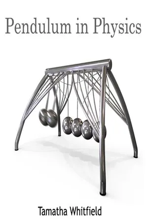
Physical Pendulum
A physical pendulum is a rigid body that can oscillate about an axis due to the force of gravity. Unlike a simple pendulum, which consists of a mass suspended by a string, a physical pendulum has a more complex shape and can exhibit different oscillation behaviors. Its motion is governed by the principles of rotational dynamics and can be analyzed using the moment of inertia and torque.
Written by Perlego with AI-assistance
Related key terms
1 of 5
5 Key excerpts on "Physical Pendulum"
 No longer available |Learn more
- (Author)
- 2014(Publication Date)
- The English Press(Publisher)
Mathematically, for small swings the pendulum approximates a harmonic oscillator, and its motion approximates to simple harmonic motion: Compound pendulum The length L of the ideal simple pendulum above, used for calculating the period, is the distance from the pivot point to the center of mass of the bob. For a real pendulum consisting of a swinging rigid body, called a compound pendulum , the length is more difficult to define. A real pendulum swings with the same period as a simple pendulum with a length equal to the distance from the pivot point to a point in the pendulum called the center of oscillation . This is located under the center of mass, at a distance called the radius of gyration, that depends on the mass distribution along the pendulum. However, for the usual sort of pendulum in which most of the mass is concentrated in the bob, the center of oscillation is close to the center of mass. ________________________ WORLD TECHNOLOGIES ________________________ Christiaan Huygens proved in 1673 that the pivot point and the center of oscillation are interchangeable. This means if any pendulum is turned upside down and swung from a pivot at the center of oscillation, it will have the same period as before, and the new center of oscillation will be the old pivot point. History One of the earliest known uses of a pendulum was in the 1st century seismometer device of Han Dynasty Chinese scientist Zhang Heng. Its function was to sway and activate one of a series of levers after being disturbed by the tremor of an earthquake far away. Released by a lever, a small ball would fall out of the urn-shaped device into one of eight metal toad's mouths below, at the eight points of the compass, signifying the direction the earthquake was located. Many sources claim that the 10th century Egyptian astronomer Ibn Yunus used a pendulum for time measurement, but this was an error that originated in 1684 with the British historian Edward Bernard. eBook - PDF
Why Toast Lands Jelly-Side Down
Zen and the Art of Physics Demonstrations
- Robert Ehrlich(Author)
- 2020(Publication Date)
- Princeton University Press(Publisher)
Discussion A light Physical Pendulum can be made from the pop-sicle stick if you make a hole at one end of the stick, and place a thin nail through the hole to serve as an axle for the pendulum. The role of the plastic ruler is 135 Mechanical Oscillations and Waves to provide an oscillating point of support for the pen-dulum. Press one end of the ruler down at the edge of a table, so that the ruler projects forward like a diving board with the pendulum at its end. Now tape the nail to the end of the ruler, so as to allow the pen-dulum to rotate freely in a vertical circle. If you put the pendulum in the inverted position, and release it, it will, of course, topple over. However, if the end of the ruler is plucked, with the pendulum initially in the inverted position, it will not topple over for a few seconds, during which the ruler vibrates with sufficient amplitude. How can we explain this strange behavior? Consider the torque on the inverted pendulum when it is a small angle 9 away from its inverted orientation: T = --mglQ, where the plus sign re-minds us that this is not a restoring torque. In the absence of ruler vibrations, Newton's second law— Id 2 d/dt 2 = +mgld —yields only divergent solutions involving exponential or hyperbolic functions of time. But, now suppose the ruler vibrates with a frequency u> 0 , so that the end of the ruler has an instantaneous acceleration asina) 0 t. In the noninertial reference frame moving with the end of the ruler, we may take the acceleration of gravity to be g + a sin g, the torque on the pendu-lum is of the restoring type (negative sign) for part of each ruler vibration. eBook - PDF
- Patrick Hamill(Author)
- 2022(Publication Date)
- Cambridge University Press(Publisher)
Note that this has the same form as the energy equation for a simple harmonic oscillator. The frequency of oscillation in η is ω = κ/ml 2 . Plugging in the expression (12.40) for κ this reproduces Equation (12.36). Therefore, the motion of a spherical pendulum with energy slightly greater than E 0 is circular motion around the vertical axis with small oscillations in θ of frequency ω. Exercise 12.11 For a spherical pendulum, show that the ratio of the angular frequencies in the azimuthal (φ) and polar (θ) directions is 1 + 3 cos 2 θ 0 . 12.5 Summary After studying this chapter you will probably agree that the “simple pendulum” is not so simple after all! One of the benefits of studying the motion of a pendulum is that it leads to a consideration of a variety of mathematical techniques. The period of a simple pendulum with arbitrary amplitude is P = 4 ω π/2 0 dφ 1 − k 2 sin 2 φ , a complete elliptic integral of the first kind. These have been tabulated but they can also be evaluated using a series expansion. An analysis of the Physical Pendulum introduces a number of properties of extended bodies, including the radius of gyration k defined in terms of the moment of inertia as I = Mk 2 . A simple pendulum oscillating with the same frequency as a Physical Pendulum has a length given by l = k 2 0 / h, where h is the distance from the axis of rotation to the center of mass, and k 0 is the radius of gyration relative to the axis. The distance l is also the distance from the axis of rotation to the center of oscillation. If a Physical Pendulum receives an impulse at the center of percussion, there will be no reaction at the axis. The center of percussion lies at the same point as the center of oscillation (but conceptually these two quantities are quite different). 12.6 Problems 343 The motion of a spherical pendulum is most easily understood by introducing an effective potential V eff = p 2 φ 2ml 2 sin 2 θ + mgl cos θ . eBook - PDF
Science Teaching
The Contribution of History and Philosophy of Science, 20th Anniversary Revised and Expanded Edition
- Michael R. Matthews(Author)
- 2014(Publication Date)
- Routledge(Publisher)
An isochronic pendulum is one in which the period of the first swing is equal to that of all subsequent swings: this implies perpetual motion. We know that any pendulum, when let swing, will very soon come to a halt: the period of the last swing will be by no means the same as the first. Furthermore, it was plain to see that cork and lead pendulums have a slightly different frequency, and that large-amplitude swings do take somewhat longer than small-amplitude swings for the same pendulum length. All of this was pointed out to Galileo, and he was reminded of Aristotle’s basic methodological claim that the evidence of the senses is to be preferred over other evidence in developing an understanding of the world. The fundamental laws of classical mechanics are not verified in experience; further, their direct verification is fundamentally impossible. Herbert Butterfield (1900–1979) conveys something of the problem that Galileo and Newton had in forging their new science: 11 They were discussing not real bodies as we actually observe them in the real world, but geometrical bodies moving in a world without resistance and without gravity History and Philosophy: Pendulum Motion 227 – moving in that boundless emptiness of Euclidean space which Aristotle had regarded as unthinkable. In the long run, therefore, we have to recognise that here was a problem of a fundamental nature, and it could not be solved by close observation within the framework of the older system of ideas – it required a transposition in the mind. (Butterfield 1949/1957, p. 5) An objectivist, non-empiricist account of science stresses that the transposi- tion in the mind is really the creation of a new theoretical object or system. Even for Galileo, the pendulum seemed to stop at the top of its swing; it was only in his theory, not his perceptual mind, that it continued in smooth motion. eBook - ePub
Experiments and Demonstrations in Physics
Bar-Ilan Physics Laboratory
- Yaakov Kraftmakher(Author)
- 2014(Publication Date)
- WSPC(Publisher)
et al (2002) observed oscillations of a pendulum with one of three damping effects: friction not depending on the velocity (sliding friction), linear dependence on the velocity (eddy currents in a metal plate), and quadratic dependence on the velocity (air friction).For other experiments with pendulums, see Lapidus (1970); Schery (1976); Hall and Shea (1977); Simon and Riesz (1979); Hall (1981); Yurke (1984); Eckstein and Fekete (1991); Ochoa and Kolp (1997); Peters (1999); Lewowski and Woźniak (2002); LoPresto and Holody (2003); Parwani (2004); Coullet et al (2005); Ng and Ang (2005); Jai and Boisgard (2007); Gintautas and Hübler (2009); Mungan and Lipscombe (2013).Theoretical background. For a mathematical pendulum with friction, the motion equation iswhere m is the mass, a is the acceleration, x is the displacement, v is the velocity, k and λ are coefficients of proportionality, x′ = v = dx/dt, and x″ = d2 x/dt2 . The solution to this equation describing free oscillations iswhere A and φ1 depend on the initial conditions. The natural frequency of the system is ω0 = (k/m)½ = (g/l)½ , the decay of free oscillations is governed by the decay constant δ = λ/2m, and the angular frequency Ω is somewhat lower than ω0 : Ω2 = ω0 2 – δ2 .The transient process after application of a periodic driving force deserves special consideration. Whenever forced oscillations start, a process occurs leading to steady oscillations. This transient process is caused by the superposition of forced and free oscillations. Landau and Lifshitz (1982) and Pippard (1989) considered the problem in detail, and this analysis is partly reproduced here. For a driven mathematical pendulum
Index pages curate the most relevant extracts from our library of academic textbooks. They’ve been created using an in-house natural language model (NLM), each adding context and meaning to key research topics.