Frequently Asked Questions in Quantitative Finance

Paul Wilmott

• Publisher: Wiley
• Year: 2010
• ISBN:
  9780470685143
• Edition: 1
• Topic: Negocios y empresa
• Subtopic: Finanzas

Getting agreement between finance theory and finance practice is important like never before. In the last decade the derivatives business has grown to a staggering size, such that the outstanding notional of all contracts is now many multiples of the underlying world economy. No longer are derivatives for helping people control and manage their financial risks from other business and industries, no, it seems that the people are toiling away in the fields to keep the derivatives market afloat! (Apologies for the mixed metaphor!) If you work in derivatives, risk, development, trading, etc. you'd better know what you are doing, there's now a big responsibility on your shoulders.

In this second edition of Frequently Asked Questions in Quantitative Finance I continue in my mission to pull quant finance up from the dumbed-down depths, and to drag it back down to earth from the super-sophisticated stratosphere. Readers of my work and blogs will know that I think both extremes are dangerous. Quant finance should inhabit the middle ground, the mathematics sweet spot, where the models are robust and understandable, and easy to mend.

…And that's what this book is about.

This book contains important FAQs and answers that cover both theory and practice. There are sections on how to derive Black-Scholes (a dozen different ways!), the popular models, equations, formulae and probability distributions, critical essays, brainteasers, and the commonest quant mistakes. The quant mistakes section alone is worth trillions of dollars!

I hope you enjoy this book, and that it shows you how interesting this important subject can be. And I hope you'll join me and others in this industry on the discussion forum on wilmott.com. See you there!"

FAQQF2...including key models, important formulae, popular contracts, essays and opinions, a history of quantitative finance, sundry lists, the commonest mistakes in quant finance, brainteasers, plenty of straight-talking, the Modellers' Manifesto and lots more.

Chapter 1

The Quantitative Finance Timeline

There follows a speedy, roller-coaster of a ride through the official history of quantitative finance, passing through both the highs and lows. Where possible I give dates, name names and refer to the original sources.²

1827 Brown The Scottish botanist, Robert Brown, gave his name to the random motion of small particles in a liquid. This idea of the random walk has permeated many scientific fields and is commonly used as the model mechanism behind a variety of unpredictable continuous-time processes. The lognormal random walk based on Brownian motion is the classical paradigm for the stock market. See Brown (1827).

1900 Bachelier Louis Bachelier was the first to quantify the concept of Brownian motion. He developed a mathematical theory for random walks, a theory rediscovered later by Einstein. He proposed a model for equity prices, a simple normal distribution, and built on it a model for pricing the almost unheard of options. His model contained many of the seeds for later work, but lay ‘dormant’ for many, many years. It is told that his thesis was not a great success and, naturally, Bachelier’s work was not appreciated in his lifetime. See Bachelier (1995).

1905 Einstein Albert Einstein proposed a scientific foundation for Brownian motion in 1905. He did some other clever stuff as well. See Stachel (1990).

1911 Richardson Most option models result in diffusion-type equations. And often these have to be solved numerically. The two main ways of doing this are Monte Carlo and finite differences (a sophisticated version of the binomial model).

The very first use of the finite-difference method, in which a differential equation is discretized into a difference equation, was by Lewis Fry Richardson in 1911, and used to solve the diffusion equation associated with weather forecasting. See Richardson (1922). Richardson later worked on the mathematics for the causes of war. During his work on the relationship between the probability of war and the length of common borders between countries he stumbled upon the concept of fractals, observing that the length of borders depended on the length of the ‘ruler.’ The fractal nature of turbulence was summed up in his poem “Big whorls have little whorls that feed on their velocity, and little whorls have smaller whorls and so on to viscosity.”

1923 Wiener Norbert Wiener developed a rigorous theory for Brownian motion, the mathematics of which was to become a necessary modelling device for quantitative finance decades later. The starting point for almost all financial models, the first equation written down in most technical papers, includes the Wiener process as the representation for randomness in asset prices. See Wiener (1923).

1950s Samuelson The 1970 Nobel Laureate in Economics, Paul Samuelson, was responsible for setting the tone for subsequent generations of economists. Samuelson ‘mathematized’ both macro and micro economics. He rediscovered Bachelier’s thesis and laid the foundations for later option pricing theories. His approach to derivative pricing was via expectations, real as opposed to the much later risk-neutral ones. See Samuelson (1955).

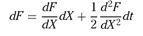
1951 Itô Where would we be without stochastic or Itô calculus? (Some people even think finance is only about Itô calculus.) Kiyosi Itô showed the relationship between a stochastic differential equation for some independent variable and the stochastic differential equation for a function of that variable. One of the starting points for classical derivatives theory is the lognormal stochastic differential equation for the evolution of an asset. Itô’s lemma tells us the stochastic differential equation for the value of an option on that asset.

In mathematical terms, if we have a Wiener process X with increments dX that are normally distributed with mean zero and variance dt, then the increment of a function F (X) is given by

This is a very loose definition of Itô’s lemma but will suffice. See Itô (1951).

1952 Markowitz Harry Markowitz was the first to propose a modern quantitative methodology for portfolio selection. This required knowledge of assets’ volatilities and the correlation between assets. The idea was extremely elegant, resulting in novel ideas such as ‘efficiency’ and ‘market portfolios.’ In this Modern Portfolio Theory, Markowitz showed that combinations of assets could have better properties than any individual assets. What did ‘better’ mean? Markowitz quantified a portfolio’s possible future performance in terms of its expected return and its standard deviation. The latter was to be interpreted as its risk. He showed how to optimize a portfolio to give the maximum expected return for a given level of risk. Such a portfolio was said to be ‘efficient.’ The work later won Markowitz a Nobel Prize for Economics but is problematic to use in practice because of the difficulty in measuring the parameters ‘volatility,’ and, especially, ‘correlation,’ and their instability.

1963 Sharpe, Lintner and Mossin William Sharpe of Stanford, John Lintner of Harvard and Norwegian economist Jan Mossin independently developed a simple model for pricing risky assets. This Capital Asset Pricing Model (CAPM) also reduced the number of parameters needed for portfolio selection from those needed by Markowitz’s Modern Portfolio Theory, making asset allocation theory more practical. See Sharpe, Alexander and Bailey (1999), Lintner (1965) and Mossin (1966).

1966 Fama Eugene Fama concluded that stock prices were unpredictable and coined the phrase ‘market efficiency.’ Although there are various forms of market efficiency, in a nutshell the idea is that stock market prices reflect all publicly available information, and that no person can gain an edge over another by fair means. See Fama (1966).

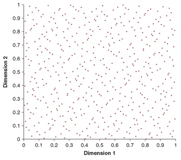
1960s Sobol’, Faure, Hammersley, Haselgrove and Halton ... Many people were associated with the definition and development of quasi random number theory or low-discrepancy sequence theory. The subject concerns the distribution of points in an arbitrary number of dimensions in order to cover the space as efficiently as possible, with as few points as possible (see Figure 1.1). The methodology is used in the evaluation of multiple integrals among other things. These ideas would find a use in finance almost three decades later. See Sobol’ (1967), Faure (1969), Hammersley & Handscomb (1964), Haselgrove (1961) and Halton (1960).

1968 Thorp Ed Thorp’s first claim to fame was that he figured out how to win at casino Blackjack, ideas that were put into practice by Thorp himself and written about in his best-selling Beat the Dealer, the “book that made Las Vegas change its rules.” His second claim to fame is that he invented and built, with Claude Shannon, the information theorist, the world’s first wearable computer. His third claim to fame is that he used the ‘correct’ formulæ for pricing options, formulæ that were rediscovered and originally published several years later by the next three people on our list. Thorp used these formulæ to make a fortune for himself and his clients in the first ever quantitative finance-based hedge fund. He proposed dynamic hedging as a way of removing more risk than static hedging. See Thorp (2002) for the story behind the discovery of the Black-Scholes formulæ.

Figure 1.1: They may not look like it, but these dots are distributed deterministically so as to have very useful properties.

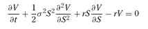
1973 Black, Scholes and Merton Fischer Black, Myron Scholes and Robert Merton derived the Black-Scholes equation for options in the early seventies, publishing it in two separate papers in 1973 (Black & Scholes, 1973, and Merton, 1973). The date corresponded almost exactly with the trading of call options on the Chicago Board Options Exchange. Scholes and Merton won the Nobel Prize for Economics in 1997. Black had died in 1995.

The Black-Scholes model is based on geometric Brownian motion for the asset price S

dS = μS dt + σ S dX .

The Black-Scholes partial differential equation for the value V of an option is then

1974 Merton, again In 1974 Robert Merton (Merton, 1974) introduced the idea of modelling the value of a company as a call option on its assets, with the company’s debt being related to the strike price and the maturity of the debt being the option’s expiration. Thus was born the structural approach to modelling risk of default, for if the option expired out of the money (i.e. assets had less value than the debt at maturity) then the firm would have to go bankrupt.

Credit risk became big, huge, in the 1990s. Theory and practice progressed at rapid speed during this period, urged on by some significant credit-led events, such as the Long Term Capital Management mess. One of the principals of LTCM was Merton who had worked on credit risk two decades earlier. Now the subject really took off, not just along the lines proposed by Merton but also using the Poisson process as the model for the random arrival of an event, such as bankruptcy or default. For a list of key research in this area see Schönbucher (2003).

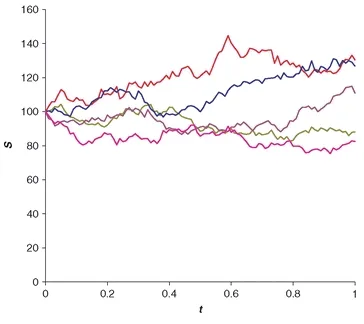
1977 Boyle Phelim Boyle related the pricing of options to the simulation of random asset paths (Figure 1.2). He showed how to find the fair value of an option by generating lots of possible future paths for an asset and then looking at the average that the option had paid off. The future important role of Monte Carlo simulations in finance was assured. See Boyle (1977).

Figure 1.2: Simulations like this can be easily used to value derivatives.

1977 Vasicek So far quantitative finance hadn’t had much to say about pricing interest rate products. Some people were using equity option formulæ for pricing interest rate options, but a consistent framework for interest rates had not been developed. This was addressed by Vasicek. He star...