An Undergraduate Introduction to Financial Mathematics

J Robert Buchanan

• Publisher: WSPC
• Year: 2012
• ISBN:
  9789814407465
• Edition: 3
• Topic: Mathématiques
• Subtopic: Mathématiques appliquées

This textbook provides an introduction to financial mathematics and financial engineering for undergraduate students who have completed a three- or four-semester sequence of calculus courses. It introduces the theory of interest, discrete and continuous random variables and probability, stochastic processes, linear programming, the Fundamental Theorem of Finance, option pricing, hedging, and portfolio optimization. This third edition expands on the second by including a new chapter on the extensions of the Black-Scholes model of option pricing and a greater number of exercises at the end of each chapter. More background material and exercises added, with solutions provided to the other chapters, allowing the textbook to better stand alone as an introduction to financial mathematics. The reader progresses from a solid grounding in multivariable calculus through a derivation of the Black-Scholes equation, its solution, properties, and applications. The text attempts to be as self-contained as possible without relying on advanced mathematical and statistical topics. The material presented in this book will adequately prepare the reader for graduate-level study in mathematical finance.

Contents:

• The Theory of Interest
• Discrete Probability
• Normal Random Variables and Probability
• The Arbitrage Theorem
• Random Walks and Brownian Motion
• Forwards and Futures
• Options
• Solution of the Black-Scholes Equation
• Derivatives of Black-Scholes Option Prices
• Hedging
• Extensions of the Black-Scholes Model
• Optimizing Portfolios
• American Options

Readership: Undergraduate students in finance, economics, and applied mathematics; professionals in banking, insurance and finance.

Chapter 1

The Theory of Interest

One of the first types of investments that people learn about is some variation on the savings account. In exchange for the temporary use of an investor's money, a bank or other financial institution agrees to pay interest, a percentage of the amount invested, to the investor. There are many different schemes for paying interest. In this chapter we will describe some of the most common types of interest and contrast their differences. Along the way the reader will have the opportunity to renew their acquaintanceship with exponential functions and the geometric series. Since an amount of capital can be invested and earn interest and thus numerically increase in value in the future, the concept of present value will be introduced. Present value provides a way of comparing values of investments made at different times in the past, present, and future. As an application of present value, several examples of saving for retirement and calculation of mortgages will be presented. Sometimes investments pay the investor varying amounts of money which change over time. The concept of rate of return can be used to convert these payments in effective interest rates, making comparison of investments easier.

1.1 Simple Interest

In exchange for the use of a depositor's money, banks pay a fraction of the account balance back to the depositor. This fractional payment is known as interest. The money a bank uses to pay interest is generated by investments and loans that the bank makes with the depositor's money. Interest is paid in many cases at specified times of the year, but nearly always the fraction of the deposited amount used to calculate the interest is called the interest rate and is expressed as a percentage paid per year. For example, a credit union may pay 6% annually on savings accounts. This means that if a savings account contains $100 now, then exactly one year from now the bank will pay the depositor $6 (which is 6% of $100) provided the depositor maintains an account balance of $100 for the entire year.

In this chapter and those that follow, interest rates will be denoted symbolically by r. To simplify the formulas and mathematical calculations, when r is used it will be converted to decimal form even though it may still be referred to as a percentage. The 6% annual interest rate mentioned above would be treated mathematically as r = 0.06 per year. The initially deposited amount which earns the interest will be called the principal amount and will be denoted P. The sum of the principal amount and any earned interest will be called the capital or the amount due. The symbol A will be used to represent the amount due. The reader may even see the amount due referred to as the compound amount, though this use of the adjective “compound” is independent of its use in the term “compound interest” to be explored in Section 1.2. The relationship between P, r, and A for a single year period is

A = P + P_r = P(1 + r).

In general, if the time period of the deposit is t years then the amount due is expressed in the formula

This implies that the average account balance for the period of the deposit is P and when the balance is withdrawn (or the account is closed), the principal amount P plus the interest earned Prt is returned to the investor. No interest is credited to the account until the instant it is closed. This is known as the simple interest formula.

Some financial institutions credit interest earned by the account balance at fixed points in time. Banks and other financial institutions “pay” the depositor by adding the interest to the depositor's account. The interest, once paid to the depositor, is the depositor's to keep. Unless the depositor withdraws the interest or some part of the principal, the process begins again for another interest earning period. If P is initially deposited, then after one year, the amount due according to Eq. (1.1) with t = 1 would be P(1 + r). This amount can be thought of as the principal amount for the account at the beginning of the second year. Thus, two years after the initial deposit the amount due would be

A = P(1 + r) + P(1 + r)r = P(1 + r)².

Continuing in this way we can see that t years after the initial deposit of an amount P, the capital A will grow to

A mathematical “purist” may wish to establish Eq. (1.2) using the principle of induction.

Banks and other interest-paying financial institutions often pay interest more than a single time per year. The yearly interest formula given in Eq. (1.2) must be modified to track the compound amount for interest periods of other than one year.

1.2 Compound Interest

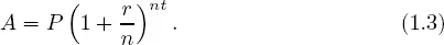
The typical interest bearing savings or checking account will be described by an investor as earning a nominal annual interest rate compounded some number of times per year. Investors will often find interest compounded semi-annually, quarterly, monthly, weekly, or daily. In this section we will compare and contrast compound interest to the simple interest case of the previous section. Whenever interest is allowed to earn interest itself, an investment is said to earn compound interest. In this situation, part of the interest is paid to the depositor once or more frequently per year. Once paid, the interest begins earning interest. We will let n denote the number of compounding periods per year. For example for interest “compounded monthly” n = 12. Only two small modifications to the interest formula in Eq. (1.2) are needed to calculate the compound interest. First, it is now necessary to think of the interest rate per compounding period. If the annual interest rate is r, then the interest rate per compounding period is r/n. Second, the elapsed time should be thought of as some number of compounding periods rather than years. Thus, with n compounding periods per year, the number of compounding periods in t years is nt. Therefore, the formula for compound interest is

Eq. (1.3) simplifies to the formula for the amount due given in Eq. (1.2) when n = 1.

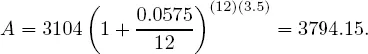
Example 1.1 Suppose an account earns 5.75% annually compounded monthly. If the principal amount is $3104 then after three and one-half years the amount due will be

The reader should verify using Eq. (1.1) th...