The Handbook of Traditional and Alternative Investment Vehicles

Investment Characteristics and Strategies

Mark J. P. Anson, Frank J. Fabozzi, Frank J. Jones

• Publisher: Wiley
• Year: 2010
• ISBN:
  9781118008690
• Edition: 1
• Topic: Business
• Subtopic: Finance
• Index: Business

A comprehensive volume that covers a complete array of traditional and alternative investment vehicles

This practical guide provides a comprehensive overview of traditional and alternative investment vehicles for professional and individual investors hoping to gain a deeper understanding of the benefits and pitfalls of using these products.

In it, expert authors Mark Anson, Frank Fabozzi, and Frank Jones clearly present the major principles and methods of investing and their risks and rewards. Along the way, they focus on providing you with the information needed to successfully invest using a host of different methods depending upon your needs and goals.

• Topics include equities, all types of fixed income securities, investment-oriented insurance products, mutual funds, closed-end funds, investment companies, exchange-traded funds, futures, options, hedge funds, private equity, and real estate
• Written by the expert author team of Mark Anson, Frank Fabozzi, and Frank Jones
• Includes valuable insights for everyone from finance professionals to individual investors

Many finance books offer collections of expertise on one or two areas of finance, but The Handbook of Traditional and Alternative Investment Vehicles brings all of these topics together in one comprehensive volume.

CHAPTER 1

Introduction

There is a wide range of financial instruments. The most general classification of financial instruments is based on the nature of the claim that the investor has on the issuer of the instrument. When the contractual arrangement is one in which the issuer agrees to pay interest and repay the amount borrowed, the financial instrument is said to be a debt instrument . In contrast to a debt instrument, an equity instrument represents an ownership interest in the entity that has issued the financial instrument. The holder of an equity instrument is entitled to receive a pro rata share of earnings, if any, after the holders of debt instruments have been paid. Common stock is an example of an equity claim. A partnership share in a business is another example.

Some financial instruments fall into both categories in terms of their attributes. Preferred stock, for example, is an equity instrument that entitles the investor to receive a fixed amount of earnings. This payment is contingent, however, and due only after payments to holders of debt instrument are made. Another hybrid instrument is a convertible bond, which allows the investor to convert a debt instrument into an equity instrument under certain circumstances. Both debt instruments and preferred stock are called fixed income instruments.

In this chapter, we’ll provide some basics about financial instruments, the general types of risks associated with investing, and characteristics of asset classes.

RISKS ASSOCIATED WITH INVESTING

There are various risks associated with investing and these will be described throughout the book. Here we will provide a brief review of the major risks associated with investing.

Total Risk

The dictionary defines risk as “hazard, peril, exposure to loss or injury.” With respect to investing, investors have used a variety of definitions to describe risk. Today, the most commonly accepted definition of risk is one that involves a well-known statistical measure known as the variance and is referred to as the total risk. The variance measures the dispersion of the outcomes around the expected value of all outcomes. Another name for the expected value is the average value.

In applying this statistical measure to the returns for a financial instrument, which we refer to as an asset for our discussion here, the observed returns on that asset over some time period are first obtained. Appendix A explains how returns for an asset are calculated. From those observed returns, the average return (which is the average or mean value) can be computed and using that average value, the variance can be computed. The square root of the variance is the standard deviation.

Despite the dominance of the variance (or standard deviation) as a measure of total risk, there are problems with using this measure to quantify the total risk for many of the assets we describe in this book. The first problem is that since the variance measures the dispersion of an asset’s return around its expected value, it considers the possibility of returns above the expected return and below the average return. Investors, however, do not view possible returns above the expected return as an unfavorable outcome. In fact, such outcomes are viewed as favorable. Because of this, it is argued that measures of risk should not consider the possible returns above the expected return. Various measures of downside risk, such as risk of loss and value at risk, are currently being used by practitioners.

The second problem is that the variance is only one measure of how the returns vary around the expected return. When a probability distribution is not symmetrical around its expected return, then another statistical measure known as skewness should be used in addition to the variance. Skewed distributions are referred to in terms of tails and mass. The tails of a probability distribution for returns is important because it is in the tails where the extreme values exist. An investor should be aware of the potential adverse extreme values for an investment and an investment portfolio. The statistical measures important for understanding risk, skewness and kurtosis, are explained in Appendix B.

Diversification

One way of reducing the total risk associated with holding an individual asset is by diversifying. Often, one hears financial advisors and professional money managers talking about diversifying their portfolio. By this it is meant the construction of a portfolio in such a way as to reduce the portfolio’s total risk without sacrificing expected return. This is certainly a goal that investors should seek. However, the question is, how does one do this in practice?

Some financial advisors and the popular press might say that a portfolio can be diversified by including assets across all asset classes. (We’ll explain in more detail what we mean by an asset class below.) Although that might be reasonable, two questions must be addressed in order to construct a diversified portfolio. First, how much of the investor’s wealth should be invested in each asset class? Second, given the allocation, which specific assets should the investor select?

Some investors who focus only on one asset class such as common stock argue that such portfolios should also be diversified. By this they mean that an investor should not place all funds in the stock of one company, but rather should include stocks of many companies. Here, too, several questions must be answered in order to construct a diversified portfolio. First, which companies should be represented in the portfolio? Second, how much of the portfolio should be allocated to the stocks of each company?

Prior to the development of portfolio theory by Harry Markowitz in 1952,¹ while financial advisors often talked about diversification in these general terms, they never provided the analytical tools by which to answer the questions posed here. Markowitz demonstrated that a diversification strategy should take into account the degree of correlation (or covariance) between asset returns in a portfolio. The correlation of asset returns is a measure of the degree to which the returns on two assets vary or change together. Correlation values range from −1 to +1.

Indeed, a key contribution of what is now popularly referred to as “Markowitz diversification” or “mean-variance diversification” is the formulation of an asset’s risk in terms of a portfolio of assets, rather than the total risk of an individual asset. Markowitz diversification seeks to combine assets in a portfolio with returns that are less than perfectly positively correlated in an effort to lower the portfolio’s total risk (variance) without sacrificing return. It is the concern for maintaining expected return while lowering the portfolio’s total risk through an analysis of the correlation between asset returns that separates Markowitz diversification from other approaches suggested for diversification and makes it more effective.

The principle of Markowitz diversification states that as the correlation between the returns for assets that are combined in a portfolio decreases, so does the variance of the portfolio’s total return. The good news is that investors can maintain expected portfolio return and lower portfolio total risk by combining assets with lower (and preferably negative) correlations. However, the bad news is that very few assets have small to negative correlations with other assets. The problem, then, becomes one of searching among a large number of assets in an effort to discover the portfolio with the minimum risk at a given level of expected return or, equivalently, the highest expected return at a given level of risk. Such portfolios are called efficient portfolios.

The recent financial market crisis has taught an important lesson about constructing efficient portfolios and what to expect from them. Specifically, when constructing a portfolio based on the historical correlations observed, there is no assurance that those correlations may not adversely change over time, particularly in stressful periods in financial markets. By “adversely change” it is meant that correlations that may be considerably less than one when designing a diversified portfolio might move closer to one. This is because during such times there are typically massive sell offs of all assets because of the concerns of a systemic threat to the financial markets throughout the world.

Systematic vs. Unsystematic Risk

The total risk of an asset or a portfolio can be divided into two types of risk: systematic risk and unsystematic risk. William Sharpe defined systematic risk as the portion of an asset’s variability that can be attributed to a common factor.² It is more popularly referred to as market risk. Because in the models developed to explain how total risk can be partitioned, the Greek letter beta was used to represent the quantity of systematic risk associated with an asset or portfolio, the term “beta” or “beta risk” has been used to mean market risk.

Systematic risk is the minimum level of risk that can be attained for a portfolio by means of diversification across a large number of randomly chosen assets. As such, systematic risk is that which results from general market and economic conditions that cannot be diversified away. For this reason the term undiversifiable risk is also used to describe systematic risk.

Sharpe defined the portion of an asset’s return variability (i.e., total risk) that can be diversified away as unsystematic risk. It is also called diversifiable risk, unique risk, residual risk, idiosyncratic risk, or company-specific risk. This is the risk that is unique to a company, such as an employee strike, the outcome of unfavorable litigation, or a natural catastrophe.

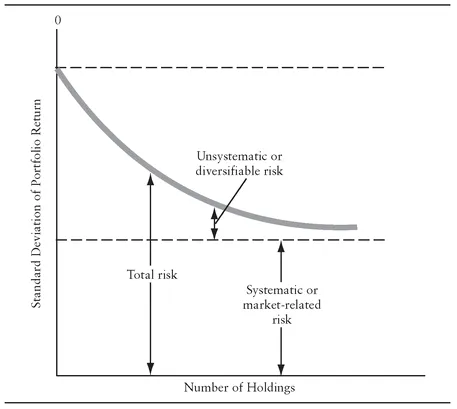
EXHIBIT 1.1 Systematic and Unsystematic Portfolio Risk

How diversification reduces unsystematic risk for portfolios is illustrated in Exhibit 1.1. The vertical axis shows the standard deviation of a portfolio’s total return. The standard deviation represents the total risk for the portfolio (systematic plus unsystematic). The horizontal axis shows the number of holdings of different assets (e.g., the number of common stock held of different companies). As can be seen, as the number of asset holdings increases (assuming that the assets are less than perfectly correlated as discussed below), the level of unsystematic risk is almost completely eliminated (that is, diversified away). The risk that remains is systematic risk. Studies of different asset classes support this. For example, for common stock, several studies suggest that a portfolio size of about 20 randomly selected companies will completely eliminate unsystematic risk leaving only systematic risk.

The relationship between the movement in the price of an asset and the market can be estimated statistically. There are two products of the estimated relationship that investors use. The first is the beta of an asset. Beta measures the sensitivity of an asset’s return to changes in the market’s return. Hence, beta is referred to as an index of systematic risk due to general market conditions that cannot be diversified away. For example, if an asset has a beta of 1.5, it means that, on average, if the market changes by 1%, the asset’s return changes by about 1.5%. The beta for the market is one. A beta that is greater than one means that systematic risk is greater than that of the market; a beta less than one means that the systematic risk is less than that of the market. Brokerage firms, vendors such as Bloomberg, Yahoo! Finance, and online Internet services provide information on beta for common stock.

The second product is the ratio of the amount of systematic risk relative to the total risk. This ratio, called the coefficient of determination or R-squared, varies from zero to one. A value of 0.8 for a portfolio means that 80% of the variation in the portfolio’s return is explained by movements in the market. For individual assets, this ratio is typically low because there is a good deal of unsystematic risk. However, as shown in Exhibit 1.1, through diversification the ratio increases as unsystematic risk is reduced.

Inflation or Purchasing Power Risk

Inflation risk, or purchasing power risk, is the potential erosion in the value of an asset’s cash flows due to inflation, as measured in terms of purchasing power. For example, if an investor purchases an asset that produces an annual return of 5% and the rate of inflation is 3%, the purchasing power of the investor has not increased by 5%. Instead, the investor’s purchasing power has increased by 2%.

Different asset classes have different exposure to inflation risk. As explained in later chapters, there are some financial instruments specifically designed to adjust for the rate of inflation.

Credit Risk

The typical definition of credit risk is that it is the risk that a borrower will fail to satisfy its financial obligations under a debt agreement. The securities issued by the U.S. Department of the Treasury are viewed as free of credit risk. (Whether this remains true in the future will depend on the U.S. government economic policies.) An investor who purchases an asset not guaranteed by the U.S. government is viewed as being exposed to credit risk. Actually, there are several forms of credit risk: default risk, downgrade risk, and spread risk. We describe these various risks in Chapter 4 and we will see that the definition of credit risk given above is for that of default risk.

Liquidity Risk

When an investor wants to sell an asset, he or she is concerned whether the price that can be obtained is close to the true value of the asset. For example, if recent trades in the market for a particular asset have been between $40 and $40.50 and market conditions have not changed, an investor would expect to sell the asset in that range.

Liquidity risk is the risk that the investor will have to sell an asset below its true value where the...