Digital Electronics

John Morris

• Publisher: Routledge
• Year: 2013
• ISBN:
  9781136076855
• Edition: 1
• Topic: Tecnología e ingeniería
• Subtopic: Ingeniería eléctrica y telecomunicaciones

An essential companion to John C Morris's 'Analogue Electronics', this clear and accessible text is designed for electronics students, teachers and enthusiasts who already have a basic understanding of electronics, and who wish to develop their knowledge of digital techniques and applications. Employing a discovery-based approach, the author covers fundamental theory before going on to develop an appreciation of logic networks, integrated circuit applications and analogue-digital conversion. A section on digital fault finding and useful ic data sheets completes the book.

1

Pulse Waveforms

Digital and analogue signals

Today the world of electronics is a mixture of analogue and digital circuitry. Many systems such as amplifiers, radios and televisions operate by using analogue signals. However, other systems such as watches, calculators and computers operate using digital signals. As time passes more and more traditional analogue systems are superseded by digital forms, notably, ni-cam digital stereo, the compact audio disc and audio cassette machines which employ digitally recorded magnetic tape. There is a significant difference between analogue waveforms or signals and those which are considered to be digital. It is a good starting point to establish clearly the difference between the two types of signal.

Analogue signals

The definition of such a waveform is one that has a continuously varying quantity (such as amplitude or frequency), with time. Two such signals are shown in Fig. 1.1(a) and 1.1(b). By studying these waveforms you may see that there are an infinite number of possible values between the minimum and maximum amplitudes.

Digital signals

A digital waveform can be divided into a finite number of levels as shown in Fig. 1.2(a), (b), (c). The waveform of Fig. 1.2(a) has seven possible levels (including 0 V) between the minimum and maximum amplitude, while those of Fig. 1.2(b) and 1.2(c) have only two levels. A morse code signal has two levels, the information is conveyed by the ‘on’ time or duration of the pulses: a short duration pulse being a ‘dot’ and a longer one a ‘dash’. The type of signal we are most concerned with however is the binary signal shown in Fig. 1.2(c) where there are two levels, the high or ‘on’ and the low or ‘off’, or as they are more commonly referred to, ‘Logic 1’ and ‘Logic 0’ respectively.

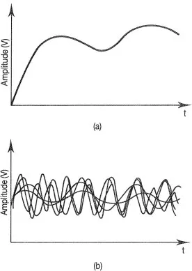
Fig. 1.1 Analogue waveforms

THOUGHT

So digital signals have specified levels and most digital systems respond to binary signals having logic levels ‘0’ and ‘1’? This is true but we must now consider the important aspects of a ‘pulse’ or ‘pulsating’ waveform.

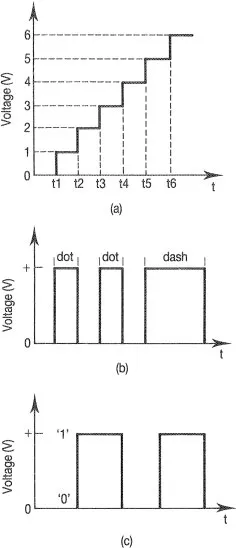
Fig. 1.2 Digital signals
(a) Seven levels
(b) Morse code
(c) Binary code

Logic gates or digital circuits of any kind respond to or are triggered by pulses, either presented singly as shown in Fig. 1.3(a) or as a ‘pulse train’ in Fig. 1.3(b). You may see from these waveforms that there are two voltage levels involved; a low voltage that represents binary ‘0’ and a higher voltage level representing binary ‘1’.

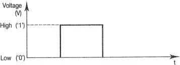
Fig. 1.3(a) Single pulse

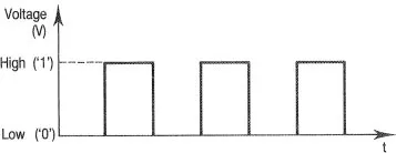
Fig. 1.3(b) Pulse train

Pulse characteristics

Having established the levels for Logic ‘1’ and ‘0’ we must now look at the pulse itself. Fig. 1.4 shows an ideal pulse as it might be displayed on the screen of an oscilloscope. You can see that the pulse appears to change from Low to High instantaneously (in zero time) and that the corners are clean cut and square. The reality is somewhat different, Fig. 1.5 shows the pulse in greater detail. Here it may be seen that there is a finite time taken for the pulse to rise from Low to High, just as it takes time for it to fall from High back to Low, and note that these times may be different. Also the corners are likely to be anything but square and will probably be curved with some ‘ringing’ or ‘overshoot’ present.

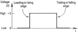
Fig. 1.4 The ideal pulse

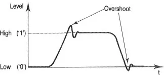
Fig. 1.5 A realistic pulse

Logic devices respond fairly quickly so that the time a pulse takes to change level is important, as is the actual duration of the pulse itself. These characteristics are indicated in Fig. 1.6.

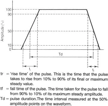
Fig. 1.6 Pulse characteristics

Pulse repetition frequency (prf)

This refers to the number of pulses that occur in one second, e.g. if the prf is 100 Hz then 100 pulses occur in 1 second. This is related to the Periodic Time (T) of the pulse.

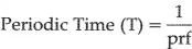
Note These definitions are similar to those you have come to know in relation to sine wave signals:

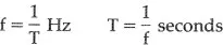
There is a great difference where pulse waveforms are concerned, however, and this can be seen by studying the waveforms of Fig. 1.7. You may notice that in both cases the periodic time (T) and hence the frequency (f) is the same. But in Fig. 1.7(a) the pulse duration is 50 s while the gap or ‘space’ between the pulses is three times as great at 150 μs. In Fig. 1.7(b) however the pulse is three times greater than the space between pulses. In both cases the frequency (f) is the same:

Fig. 1.7 Pulse repetition frequency waveforms

When considering pulse waveforms it is important that the duration of the pulse itself is quoted together with the time between pulses. This may be achieved in two ways.

The Mark to Space Ratio

With reference to Fig. 1.8, the ‘on’ time or pulse duration is termed the ‘mark’ time; and the ‘off’ time or space between pulses is termed the ‘space’ time. The ratio of pulse ‘on’ to pulse ‘off’ time is the mark to space ratio:

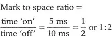
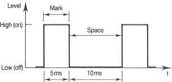
Fig. 1.8 Mark to space r...