Op Amps: Design, Application, and Troubleshooting

David Terrell

• Publisher: Newnes
• Year: 1996
• Print ISBN: 9780750697026
• eBook ISBN: 9780080513089
• Edition: 2
• Topic: Technology & Engineering
• Subtopic: Electrical Engineering & Telecommunications
• Index: Technology & Engineering

OP Amps deliberately straddles that imaginary line between the technician and engineering worlds. Topics are carefully addressed on three levels: operational overview, numerical analysis, and design procedures. Troubleshooting techniques are presented that rely on the application of fundamental electronics principles. Systematic methods are shown that can be used to diagnose defects in many kinds of circuits that employ operational amplifiers. One of the book's greatest strengths is the easy-to-read conversational writing style. The author speaks directly to the student in a manner that encourages learning. This book explains the technical details of operational amplifier circuits in clear and understandable language without sacrificing technical depth. - Easy-to-read conversational style communicates procedures an technical details in simple language - Three levels of technical material: operational overview, manericall analysis, and design procedures - Mathematics limited to algebraic manipulation

CHAPTER ONE

Basic Concepts of the Integrated Operational Amplifier

1.1 OVERVIEW OF OPERATIONAL AMPLIFIERS

1.1.1 Brief History

Operational amplifiers began in the days of vacuum tubes and analog computers. They consisted of relatively complex differential amplifiers with feedback. The circuit was constructed such that the characteristics of the overall amplifier were largely determined by the type and amount of feedback. Thus the complex differential amplifier itself had become a building block that could function in different “operations” by altering the feedback. Some of the operations that were used included adding, multiplying, and logarithmic operations.

The operational amplifier continued to evolve through the transistor era and continued to decrease in size and increase in performance. The evolution continued through molded or modular devices and finally in the mid 1960s a complete operational amplifier was integrated into a single integrated circuit (IC) package. Since that time, the performance has continued to improve dramatically and the price has generally decreased as the benefits of high-volume production have been realized. The performance increases include such items as higher operating voltages, lower current requirements, higher current capabilities, more tolerance to abuse, lower noise, greater stability, greater power output, higher input impedances, and higher frequencies of operation.

In spite of all the improvements, however, the high-performance, integrated operational amplifier of today is still based on the fundamental differential amplifier. Although the individual components in the amplifier are not accessible to you, it will enhance your understanding of the op amp if you have some appreciation for the internal circuitry.

1.1.2 Review of Differential Voltage Amplifiers

You will recall from your basic electronics studies that a differential amplifier has two inputs and either one or two outputs. The amplifier circuit is not directly affected by the voltage on either of its inputs alone, but it is affected by the difference in voltage between the two inputs. This difference voltage is amplified by the amplifier and appears in the output in its amplified form. The amplifier may have a single output, which is referenced to common or ground. If so, it is called a single-ended amplifier. On the other hand, the output of the amplifier may be taken between two lines, neither of which is common or ground. In this case, the amplifier is called a double-ended or differential output amplifier.

Figure 1.1 shows a simple transistor differential voltage amplifier. More specifically, it is a single-ended differential amplifier. The transistors have a shared emitter bias so the combined collector current is largely determined by the −20-volt source and the 10-kilohm emitter resistor. The current through this resistor then divides (Kirchhoff’s Current Law) and becomes the emitter currents for the two transistors. Within limits, the total emitter current remains fairly constant and simply diverts from one transistor to the other as the signal or changing voltage is applied to the bases. In a practical differential amplifier, the emitter network generally contains a constant current source.

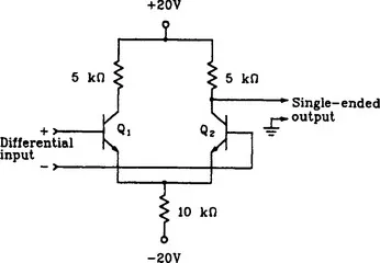
FIGURE 1.1 A simple differential voltage amplifier based on transistors.

Now consider the relative effect on the output if the input signal is increased with the polarity shown. This will decrease the bias on Q₂ while increasing the bias on Q₁. Thus a larger portion of the total emitter current is diverted through Q₁ and less through Q₂. This decreased current flow through the collector resistor for Q₂ produces less voltage drop and allows the output to become more positive.

If the polarity of the input were reversed, then Q₂ would have more current flow and the output voltage would decrease (i.e., become less positive).

Suppose now that both inputs are increased or decreased in the same direction. Can you see that this will affect the bias on both of the transistors in the same way? Since the total current is held constant and the relative values for each transistor did not change, then both collector currents remain constant. Thus the output does not reflect a change when both inputs are altered in the same way. This latter effect gives rise to the name differential amplifier. It only amplifies the difference between the two inputs, and is relatively unaffected by the absolute values applied to each input. This latter effect is more pronounced when the circuit uses a current source in the emitter circuit.

In certain applications, one of the differential inputs is connected to ground and the signal to be amplified is applied directly to the remaining input. In this case the amplifier still responds to the difference between the two inputs, but the output will be in or out of phase with the input signal depending on which input is grounded. If the signal is applied to the (+) input, with the (−) input grounded, as labeled in Figure 1.1, then the output signal is essentially in phase with the input signal. If, on the other hand, the (+) input is grounded and the input signal is applied to the (−) input, then the output is essentially 180 degrees out of phase with the input signal. Because of the behavior described, the (−) and (+) inputs are called the inverting and noninverting inputs, respectively.

1.1.3 A Quick Look Inside the IC

Figure 1.2 shows the schematic diagram of the internal circuitry for a common integrated circuit op amp. This is the 741 op amp which is common in the industry. It is not particularly important for you to understand the details of the internal operation. Nor is it worth your while to trace current flow through the internal components. The internal diagram is shown here for the following reasons:

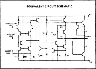
FIGURE 1.2 The internal schematic for an MC1741 op amp. (Copyright of Motorola, Inc. Used by...

Table of contents

• Cover image
• Title page
• Table of Contents
• Copyright
• Dedication
• PREFACE
• ACKNOWLEDGMENTS
• Chapter 1: Basic Concepts of the Integrated Operational Amplifier
• Chapter 2: Amplifiers
• Chapter 3: Voltage Comparators
• Chapter 4: Oscillators
• Chapter 5: Active Filters
• Chapter 6: Power Supply Circuits
• Chapter 7: Signal Processing Circuits
• Chapter 8: Digital-to-Analog and Analog-to-Digital Conversion
• Chapter 9: Arithmetic Function Circuits
• Chapter 10: Nonideal Op Amp Characteristics
• Chapter 11: Specialized Devices
• Appendices
• Index