Vascular Imaging of the Central Nervous System

Physical Principles, Clinical Applications, and Emerging Techniques

Joana Ramalho, Mauricio Castillo

• Publisher: Wiley-Blackwell
• Year: 2013
• ISBN:
  9781118434383
• Edition: 1
• Topic: Medicine
• Subtopic: Radiology, Radiotherapy & Nuclear Medicine

The first book-length reference to thoroughly describe diagnostic and therapeutic advances in the development of vascular radiology over the last decade

The last ten years has seen vascular imaging of the central nervous system (CNS) evolve from fairly crude, invasive procedures to more advanced imaging methods that are safer, faster, and more precise—with computed tomographic (CT) and magnetic resonance (MR) imaging methods playing a special role in these advances.

Vascular Imaging of the Central Nervous System is the first full-length reference text that shows radiologists—especially neuroradiologists—how to optimize the use of the many techniques available in order to increase the sensitivity and specificity of vascular imaging, thereby improving the diagnosis and treatment of individual patients. Each chapter is formatted carefully and divided into two essential parts: The first part describes the physical principles underlying each imaging technique, along potential associated artifacts and pitfalls; the second part addresses clinical applications and novel applications of each method.

With a strong focus on the clinical application of each modality or technique in CNS radiology, this book provides in-depth chapter coverage of:

•Ultrasound Vascular Imaging (UVI)
•Computed Tomography Angiography (CTA)
•Magnetic Resonance Vascular imaging (MRV)
•Digital subtraction angiography (DSA)
•Brain perfusion techniques: CT and MRI
•Plaque imaging
•Intravascular imaging
•Pediatric vascular imaging

Along with numerous illustrations and case studies, Vascular Imaging of the Central Nervous System: Physical Principles, Clinical Applications, and Emerging Techniques is an important book for those faced with choosing from the wide range of choices available for clinical practice.

One

Ultrasound Vascular Imaging (UVI)

1

Basic Principles of Ultrasound Sonography

Ana Maria Braz, Jaime Leal Pamplona and Joana N. Ramalho

Department of Neuroradiology, Centro Hospitalar Lisboa Central, Lisboa, Portugal

Introduction

Ultrasound imaging was first applied for medical purposes in the 1940s by Dr. Karl Theodore Dussik [1], and since then, it has spread all over the world as one of many noninvasive techniques by which we can gather information about tissues, cavities, and blood flow in the human body. It is an old technique but has a good cost–benefit ratio.

The main aim of this chapter is to provide a brief overview of the physics and instrumentation of ultrasound and Doppler imaging.

Sound

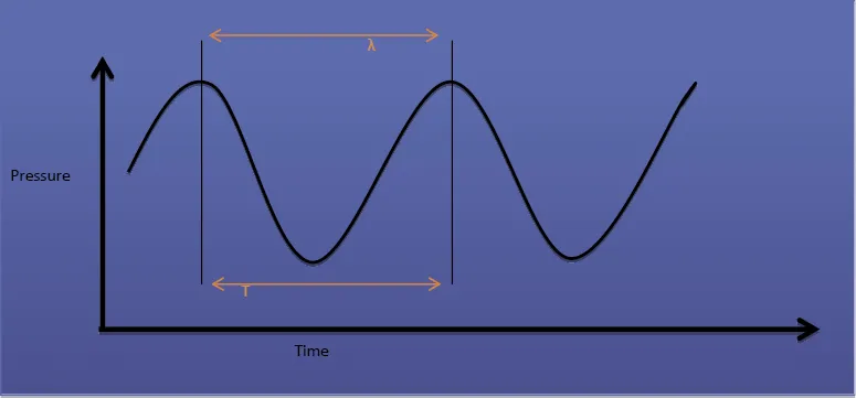
The main basic instrument of ultrasound is the sound itself. We can define sound as a sinusoidal wave that is an oscillation of pressures, transmitted through different tissues. This implies that sound mechanical energy will make a physical displacement of molecules through its passage, causing different types of rarefaction and compression in medium. In Figure 1.1, it is possible to see a sinusoidal wave, where the distance between two peak points is the wavelength (λ), the time corresponding to a complete cycle is a period (T), and frequency (f) is the number of complete cycles per second (f = 1 / T). The frequency of ultrasounds used in medicine ranges between 1 and 20 MHz, where hertz (Hz) corresponds to a cycle per second.

Figure 1.1 Sound wave. The graphic represents oscillating pressure producing compression and rarefaction of the medium. λ: wavelength, the distance between two peaks in the sine wave; T: period, the time of one cycle.

The velocity of sound in the medium is given by the equation c = f × λ, and it is determined by the density and stiffness of the medium, being directly proportional to both. Each tissue has its constant propagation velocity, and does not change by wavelength or frequency of the emitted sound. Medical ultrasound devices assume an average propagation velocity of 1540 m/s [2, 3, 4, 5].

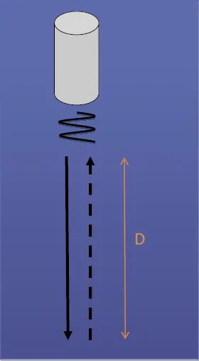
These concepts are extremely important because we are going to collect information about the depth and size of structures by using the principles of echo ranging and doing some calculus. In ultrasound, in order to obtain distance, this equation is used: d = c × t / 2, where d is distance, c is propagation velocity, and t is the time that the ultrasound signal takes to make a round trip from the transmitter, reaching the target and coming back to the receiver (Figure 1.2).

Figure 1.2 Ultrasound detection. An impulse wave is started by the transducer, goes through the medium, reaches the desired target and is reflected until the transducer. D: Distance between transducer and target.

After applying an ultrasound pulse, the time that echo returning takes is measured, and, when the propagation velocity sound for that tissue is known, the depth of the interface is calculated. This measurement is influenced not only by the accuracy of the value that is given for propagation velocity from tissue, but also by the path that sound pulses travel.

Sound amplitude is represented by the height of the wave and can be described in decibels (dB), which do not represent an absolute signal level but a logarithmic ratio of two amplitudes (A2 and A1). By halving the amplitude, the decibel's level goes up by six (dB = 20 log (A2 / A1)).

Medium

In clinical use, ultrasound images are formed by echoes (reflected sound), and to do this, there must be tissue with reflecting capability. If the medium is totally homogeneous, there won't be a reflected sound, so it will look like a cyst – in other words, an anechoic medium. At junctions of tissues with different properties, the sound will reflect, and different intensities of echoes will return. The amount of reflection (or backscatter) is called acoustic impedance (Z), and it is determined by tissue density (ρ) and the propagation velocity of the tissue (c) (Z = ρ × c). These reflections are determined by the differences between the values of each tissue's acoustic impedance. This means that a big difference in a tissue's acoustic impedance (like bone and air) will reflect almost all sounds, and smaller ones (between fat and muscle) will reflect only some sound while the other amount will continue forward through the other tissues ahead. Therefore, it is possible to say that ultrasound does not give images of tissue structures but, alternatively, interfaces between tissues with different levels of acoustic impedance.

Interface of reflection

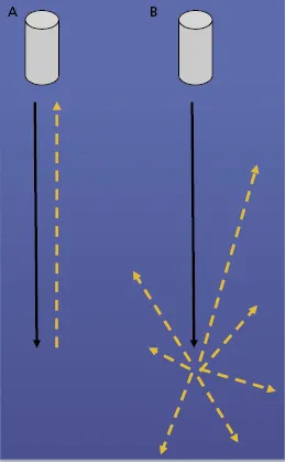
There are two types of reflection interfaces, specular reflectors and diffuse reflectors. The first one acts like a flat mirror, and the second one acts like a mirror ball (i.e., a “disco ball”). This happens because of the surface and size of the interface: if it is large and smooth (like a diaphragm or the wall of a urine-filled bladder), it will be a specular reflector, whereas if it is small and wrinkled (like the liver parenchyma), it will be a diffuse reflector. The first one will reflect, and the second one will scatter (Figure 1.3).

Figure 1.3 Specular (A) and diffuse (B) reflectors. In specular reflectors, the sound is reflected by a “flat mirror” coming straight to the transducer, if the beam was at a 90° angle. In diffuse reflectors, the sound is scatter in all direction, returning just a small amount to the transducer.

The reflection coefficient (R) is the energy reflected as a fraction of the incident energy, where Z₁ is proximal tissue impedance and Z₂ distal tissue impedance (R = (Z₂ − Z₁)² / (Z₂ + Z₁)²).

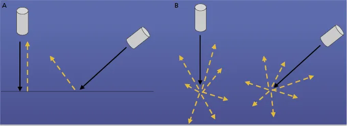
Because the specular reflector acts as a flat mirror, the returned echo depends on the degree of insonation. If the angle is too far away from a 90° angle, the sound will reflect and won't be detected by the transducer. This is very important because the ultrasound image is reconstructed only by the reflections that return to the transducer, so if the echo does not return, there won't be a good interface for images. In fact, most of the echoes come from the diffuse reflector. These interfaces produce a speckle on the ultrasound, resulting from a constructive and destructive interference of the reflected sound, directing away almost all energy with only a small part reflected toward the ultrasound transducer. Because of this property, the ultrasound incident angle does not change the amount of echo recognized (Figure 1.4). Thus, when analyzing vessels, if the wall is the main purpose of the study, it should be insonated at a 90° angle; otherwise, when studying flow in Doppler imaging, this angle should be less.

Figure 1.4 The incidence beam and the type of reflector.

Refraction is the alteration trajectory of ultrasound wave when it passes through different tissues with different acoustic propagation velocity. This means that not all echoes received in a transducer come from a straight line; they could come from a different depth or location, changing the liability of the image displayed (Figure 1.5). To reduce this artifact, the emitted ultrasound angle should be (as much as possible) perpendicular to the interface under study. Snell's law is the equation that relates the angle of refraction and propagation velocity (Sin θ₁ / sin θ₂ = c₁ / c₂).

Figure 1.5 Different tissues have different propagation velocities, leading to changes in the direction of the sound wave – refraction.

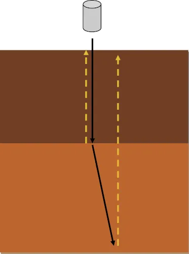
If we think of sound as an acoustic energy, while it passes through different interfaces, it will decrease wave amplitude by transferring some of that energy as heat to the ambient surrounding it – absorption – and it will reflect and scatter the rest.

The amount of energy produced in time is called acoustic power (expressed in watts [W]); and, when the energy is related in spatial distribution, it is called intensity (I) (I = W / cm²).

So attenuation is the medium capacity of decreasing ultrasound signal amplitude, which means that determines the ultrasound penetration efficiency. It is measured in decibels (dB), allowing one to compare different levels of ultrasound intensity, and is calculated by this formula: dB = 10 × log₁₀ I.

Attenuation is a result of the combined effects of absorption, scattering, and reflection, and it depends not only on the property of the medium but also on the insonating frequency. Higher emitted frequencies result in less penetration because attenuation is more pronounced:

where α is the attenuation coefficient of a tissue, L is medium length, and f is frequency.

Greater penetrations depths are achieved by using transducers with lower transmit frequencies or increasing amplification of the signal. This amplification is known as time-gain compensation or depth-gain compensation. The gain is chosen according to the depth and localization of the study vessel, and it is crucial for acquiring a signal with good amplitude and intensity. Together with the output energy and signal-to-noise limit, it is a parameter of great importance to be managed by the operator.

Doppler ultrasound

The study of blood vessels is based on the Doppler effect, which was ...

Table of contents

• Cover
• Dedication
• Title page
• Copyright page
• List of Contributors
• Preface
• Acknowledgments
• Part One: Ultrasound Vascular Imaging (UVI)
• Part Two: Computed Tomography Angiography (CTA)
• Part Three: Magnetic Resonance Vascular Imaging (MRV)
• Part Four: Digital Subtraction Angiography (DSA)
• Part Five: Brain Perfusion Techniques: Computed Tomography (CT) and Magnetic Resonance Imaging (MRI)
• Part Six: Plaque Imaging
• Part Seven: Intravascular Imaging
• Part Eight: Pediatric Vascular Imaging
• Index