Quantile Regression

Theory and Applications

Cristina Davino, Marilena Furno, Domenico Vistocco

• Publisher: Wiley
• Year: 2013
• ISBN:
  9781118752715
• Edition: 1
• Topic: Matemáticas
• Subtopic: Probabilidad y estadística

A guide to the implementation and interpretation of Quantile Regression models

This book explores the theory and numerous applications of quantile regression, offering empirical data analysis as well as the software tools to implement the methods.

The main focus of this book is to provide the reader with a comprehensive description of the main issues concerning quantile regression; these include basic modeling, geometrical interpretation, estimation and inference for quantile regression, as well as issues on validity of the model, diagnostic tools. Each methodological aspect is explored and followed by applications using real data.

Quantile Regression:

• Presents a complete treatment of quantile regression methods, including, estimation, inference issues and application of methods.
• Delivers a balance between methodolgy and application
• Offers an overview of the recent developments in the quantile regression framework and why to use quantile regression in a variety of areas such as economics, finance and computing.
• Features a supporting website ( www.wiley.com/go/quantile_regression ) hosting datasets along with R, Stata and SAS software code.

Researchers and PhD students in the field of statistics, economics, econometrics, social and environmental science and chemistry will benefit from this book.

1

A visual introduction to quantile regression

Introduction

Quantile regression is a statistical analysis able to detect more effects than conventional procedures: it does not restrict attention to the conditional mean and therefore it permits to approximate the whole conditional distribution of a response variable.

This chapter will offer a visual introduction to quantile regression starting from the simplest model with a dummy predictor, moving then to the simple regression model with a quantitative predictor, through the case of a model with a nominal regressor.

The basic idea behind quantile regression and the essential notation will be discussed in the following sections.

1.1 The essential toolkit

Classical regression focuses on the expectation of a variable Y conditional on the values of a set of variables X, E(Y|X), the so-called regression function (Gujarati 2003; Weisberg 2005). Such a function can be more or less complex, but it restricts exclusively on a specific location of the Y conditional distribution. Quantile regression (QR) extends this approach, allowing one to study the conditional distribution of Y on X at different locations and thus offering a global view on the interrelations between Y and X. Using an analogy, we can say that for regression problems, QR is to classical regression what quantiles are to mean in terms of describing locations of a distribution.

QR was introduced by Koenker and Basset (1978) as an extension of classical least squares estimation of conditional mean models to conditional quantile functions. The development of QR, as Koenker (2001) later attests, starts with the idea of formulating the estimation of conditional quantile functions as an optimization problem, an idea that affords QR to use mathematical tools commonly used for the conditional mean function.

Most of the examples presented in this chapter refer to the Cars93 dataset, which contains information on the sales of cars in the USA in 1993, and it is part of the MASS R package (Venables and Ripley 2002). A detailed description of the dataset is provided in Lock (1993).

1.1.1 Unconditional mean, unconditional quantiles and surroundings

In order to set off on the QR journey, a good starting point is the comparison of mean and quantiles, taking into account their objective functions. In fact, QR generalizes univariate quantiles for conditional distribution.

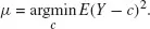
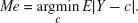
The comparison between mean and median as centers of an univariate distribution is almost standard and is generally used to define skewness. Let Y be a generic random variable: its mean is defined as the center c of the distribution which minimizes the squared sum of deviations; that is as the solution to the following minimization problem:

(1.1)

The median, instead, minimizes the absolute sum of deviations. In terms of a minimization problem, the median is thus:

(1.2)

Using the sample observations, we can obtain the sample estimators

and

for such centers.

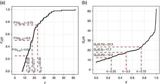
It is well known that the univariate quantiles are defined as particular locations of the distribution, that is the θ-th quantile is the value y such that P(Y ≤ y) = θ. Starting from the cumulative distribution function (CDF):

(1.3)

the quantile function is defined as its inverse:

(1.4)

for θ ∈ [0, 1]. If F (.) is strictly increasing and continuous, then F⁻¹ (θ) is the unique real number y such that F(y) = θ (Gilchrist 2000). Figure 1.1 depicts the empirical CDF [Figure 1.1(a)] and its inverse, the empirical quantile function [Figure 1.1(b)], for the Price variable of the Cars93 dataset. The three quartiles, θ = {0.25, 0.5, 0.75}, represented on both plots point out the strict link between the two functions.

Figure 1.1 Empirical distribution function (a) and its inverse, the empirical quantile function (b), for the Price variable of the Cars93 dataset. The three quartiles of Price are represented on the two plots: q_θ corresponds to the abscissa on the F_Y(y) plot, while it corresponds to the ordinate on the Q_Y(θ) plot; the other input being the value of θ.

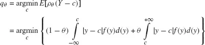
Less common is the presentation of quantiles as particular centers of the distribution, minimizing the weighted absolute sum of deviations (Hao and Naiman 2007). In such a view the θ-th quantile is thus:

(1.5)

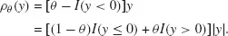
where ρ_θ (.) denotes the following loss function:

Such loss function is then an asymmetric absolute loss function; that is a weighted sum of absolute deviations, where a (1 − θ) weight is assigned to the negative deviations and a θ weight is used for the positive deviations.

In the case of a discrete variable Y with probability distribution f (y) = P(Y = y), the previous minimization problem becomes:

The same criterion is adopted in the case of a continuous random variable substituting summation with integrals:

where f (y) denotes the probability density function of Y. The sample estimator

for θ ∈ [0, 1] is likewise obtained using the sample information in the previous formula. Finally, it is straightforward to say that for θ = 0.5 we obtain the median solution defined in Equation (1.2).

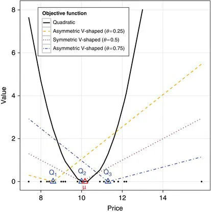
A graphical representation of these concepts is shown in Figure 1.2, where, for the subset of small cars according to the Type variable, the mean and the three quartiles for the Price variable of the Cars93 dataset are represented on the x-axis, along with the original data. The different objective function for the mean and the three quartiles are shown on the y-axis. The quadratic shape of the mean objective function is opposed to the V-shaped objective functions for the three quartiles, symmetric for the median case and asymmetric (and opposite) for the case of the two extreme quartiles.

Figure 1.2 Comparison of mean and quartiles as location indexes of a univariate distribution. Data refer to the Price of small cars as defined by the Type variable (Cars93 dataset). The car prices are represented using dots on the x-axis while the positions of the mean and of the three quartiles are depicted using triangles. Objective functions associated with the three measures are shown on the y-axis. From this figure, it is evident that the mean objective function has a quadratic shape while the quartile objective functions are V-shaped; moreover it is symmetric for the median case and asymmetric in the case of the two extreme quartiles.

1.1.2 Technical insight: Quantiles as solutions of a minimization problem

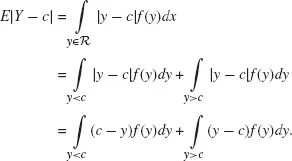
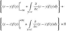
In order to show the formulation of univariate quantiles as solutions of the minimization problem (Koenker 2005) specified by Equation (1.5), the presentation of the solution for the median case, Equation (1.2), is a good starting point. Assuming, without loss of generality, that Y is a continuous random variable, the expected value of the absolute sum of deviations from a given center c can be split into the following two terms:

Since the absolute value is a convex function, differentiating E|Y − c| with respect to c and setting the partial derivatives to zero will lead to the solution for the minimum:

The solution can then be obtained applying the derivative and integrating per part as follows:

Taking into account that:

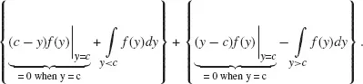
for a well-defined probability density function, the integrand restricts in y = c¹:

Using then the CDF definition, Equation (1.3), the previous equation reduces to:

and thus:

The solution of the minimization problem formulated in Equation (1.2) is thus the median. The above solution does not change by multiplying the two components of E|Y − c| by a constant θ and (1 − θ), respectively. This a...

Table of contents

• Cover
• Title page
• Copyright page
• Series1
• Preface
• Acknowledgements
• Introduction
• Nomenclature
• 1 A visual introduction to quantile regression
• 2 Quantile regression: Understanding how and why
• 3 Estimated coefficients and inference
• 4 Additional tools for the interpretation and evaluation of the quantile regression model
• 5 Models with dependent and with non-identically distributed data
• 6 Additional models
• Appendix A Quantile regression and surroundings using R
• Appendix B Quantile regression and surroundings using SAS
• Appendix C Quantile regression and surroundings using Stata
• Index
• Series2