Electrical Conduction in Graphene and Nanotubes

Shigeji Fujita, Akira Suzuki

• Publisher: Wiley-VCH
• Year: 2013
• ISBN:
  9783527676705
• Edition: 1
• Topic: Sciences physiques
• Subtopic: Matière condensée

Written in a self-contained manner, this textbook allows both advanced students and practicing applied physicists and engineers to learn the relevant aspects from the bottom up. All logical steps are laid out without omitting steps.
The book covers electrical transport properties in carbon based materials by dealing with statistical mechanics of carbon nanotubes and graphene - presenting many fresh and sometimes provoking views. Both second quantization and superconductivity are covered and discussed thoroughly. An extensive list of references is given in the end of each chapter, while derivations and proofs of specific equations are discussed in the appendix.
The experienced authors have studied the electrical transport in carbon nanotubes and graphene for several years, and have contributed relevantly to the understanding and further development of the field. The content is based on the material taught by one of the authors, Prof Fujita, for courses in quantum theory of solids and quantum statistical mechanics at the University at Buffalo, and some topics have also been taught by Prof. Suzuki in a course on advanced condensed matter physics at the Tokyo University of Science.
For graduate students in physics, chemistry, electrical engineering and material sciences, with a knowledge of dynamics, quantum mechanics, electromagnetism and solid-state physics at the senior undergraduate level. Includes a large numbers of exercise-type problems.

Chapter 1

Introduction

1.1 Carbon Nanotubes

Graphite and diamond are both made of carbons. They have different lattice structures and different properties. Diamond is brilliant and it is an insulator while graphite is black and it is a good conductor.

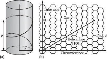
In 1991 Iijima [1] discovered carbon nanotubes (CNTs) in the soot created in an electric discharge between two carbon electrodes. These nanotubes ranging from 4 to 30 nm in diameter were found to have helical multiwalled structures as shown in Figures 1.1 and 1.2 after electron diffraction analysis. The tube length is about 1 μm.

Figure 1.1 Schematic diagram showing (a) a helical arrangement of graphitic carbons and (b) its unrolled plane. The helical line is indicated by the heavy line passing through the centers of the hexagons.

Figure 1.2 A multiwalled nanotube. The tube diameter ranges from 4 to 30 nm and its length is about 1 μm. (Original figure, lijima [1])

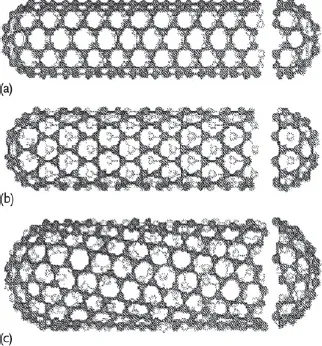
The scroll-type tube shown in Figure 1.2 is called a multiwalled carbon nanotube (MWNT). A single-wall nanotube (SWNT) was fabricated by Iijima and Ichihashi [2] and by Bethune et al. [3] in 1993. Their structures are shown in Figure 1.3.

Figure 1.3 SWNTs with different chiralities and possible caps at each end: (a) shows a so-called armchair carbon nanotube (CNT), (b) a zigzag CNT, and (c) a general chiral CNT. One can see from the figure that the orientation of the C-hexagon in the honeycomb lattice relative to the tube axis can be taken arbitrarily. The terms “armchair” and “zigzag” refer to the arrangement of C-hexagons around the circumference.

(From [4, 5]).

The tube is about 1 nm in diameter and a few micrometers in length. The tube ends are closed as shown. Because of their small radius and length-to-diameter ratio > 10⁴, they provide an important system for studying two-dimensional (2D) physics, both theoretically and experimentally. Unrolled carbon sheets are called graphene.¹⁾ They have a honeycomb lattice structure as shown in Figure 1.1b.

A SWNT can be constructed from a slice of graphene (that is a single planar layer of the honeycomb lattice of graphite) rolled into a circular cylinder.

Carbon nanotubes are light since they are entirely made of the light element carbon (C). They are strong and have excellent elasticity and flexibility. In fact, carbon fibers are used to make tennis rackets, for example. Their main advantages in this regard are their high chemical stability as well as their strong mechanical properties.

Today’s semiconductor technology is based mainly on silicon (Si). It is said that carbon-based devices are expected to be as important or even more important in the future. To achieve this purpose we must know the electrical transport properties of CNTs, which are very puzzling, as is explained below. The principal topics in this book are the remarkable electrical transport properties in CNTs and graphene on which we will mainly focus in the text.

The conductivity σ in individual CNTs varies, depending on the tube radius and the pitch of the sample. In many cases the resistance decreases with increasing temperature. In contrast the resistance increases in the normal metal such as copper (Cu). The electrical conduction properties in SWNTs separates samples into two classes: semiconducting or metallic. The room-temperature conductivities are higher for the latter class by two or more orders of magnitude. Saito et al. [6] proposed a model based on the different arrangements of C-hexagons around the circumference, called the chiralities. Figure 1.3a–c show an armchair, zigzag, and a general chiral CNT, respectively. After statistical analysis, they concluded that semiconducting SWNTs should be generated three times more often than metallic SWNTs. Moriyama et al. [7] fabricated 12 SWNT devices from one chip, and observed that two of the SWNT samples were semiconducting and the other ten were metallic, a clear discrepancy between theory and experiment. We propose a new classification. The electrical conduction in SWNTs is either semiconducting or metallic depending on whether each pitch of the helical line connecting the nearest-neighbor C-hexagon contains an integral number of hexagons or not. The second alternative (metallic SWNT) occurs more often since the helical angle between the helical line and the tube axis is not controlled in the fabrication process. In the former case the system (semiconducting SWNT) is periodic along the tube length and the “holes” (and not “electrons”) can travel along the wall. Here and in the text “electrons” (“holes”), by definition, are quasielectrons which are excited above (below) the Fermi energy and which circulate clockwise (counterclockwise) when viewed from the tip of the external magnetic field vector. “Electrons” (“holes”) are generated in the negative (positive) side of the Fermi surface which contains the negative (positive) normal vector, with the convention that the positive normal points in the energy-increasing direction. In the Wigner-Seitz (WS) cell model [7] the primitive cell for the honeycomb lattice is a rhombus. This model is suited to the study of the ground state of graphene. For the development of the electron dynamics it is necessary to choose a rectangular unit cell which allows one to define the effective masses associated with the motion of “electrons” and “holes” in the lattice.

Silicon (Si) (germanium (Ge)) forms a diamond lattice which is obtained from the zinc sulfide (ZnS) lattice by disregarding the species. The electron dynamics of Si are usually discussed in terms of cubic lattice languages. Graphene and graphite have hexagonal lattice structures. Silicon and carbon are both quadrivalent materials but because of their lattice structures, they have quite different physical properties.

1.2 Theoretical Background

1.2.1 Metals and Conduction Electrons

A metal is a conducting crystal in which electrical current can flow with little resistance. This electrical current is generated by moving electrons. The electron has mass m and charge −e, which is negative by convention. Their numerical values are m = 9.1 × 10⁻²⁸ g and e = 4.8 × 10⁻¹⁰ esu = 1.6 × 10⁻¹⁹ C. The electron mass is about 1837 times smaller than the least-massive (hydrogen) atom. This makes the electron extremely mobile. It also makes the electron’s quantum nature more pronounced. The electrons participating in the transport of charge are called conduction electrons. The conduction electrons would have orbited in the outermost shells surrounding the atomic nuclei if the nuclei were separated from each other. Core electrons which are more tightly bound with the nuclei form part of the metallic ions. In a pure crystalline metal, these metallic ions form a relatively immobile array of regular spacing, called a lattice. Thus, a metal can be pictured as a system of two components: mobil electrons and relatively immobile lattice ions.

1.2.2 Quantum Mechanics

Electrons move following the quantum laws of motion. A thorough understanding of quantum theory is essential. Dirac’s formulation of quantum theory in his book, Principles of Quantum Mechanics [9], is unsurpassed. Dirac’s rules that the quantum states are represented by bra or ket vectors and physical observables by Hermitian operators are used in the text. There are two distinct quantum effects, the first of which concerns a single particle and the second a system of identical particles.

1.2.3 Heisenberg Uncertainty Principle

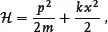
Let us consider a simple harmonic oscillator characterized by the Hamiltonian

(1.1)

where m is the mass, k the force constant, p the momentum, and x the position. The corresponding energy eigenvalues are

(1.2)

The energies are quantized in (1.2). In contrast the classical energy can be any positive value. The lowest quantum energy ε₀ = ħω₀/2, called the energy of zero-point motion, is not zero. The most stable state of any quantum system is not a state of static equilibrium in the configuration of lowest potential energy, it is rather a dynamic equilibrium for the zero-p...

Table of contents

• Cover
• Half Title page
• Title page
• Copyright page
• Preface
• Physical Constants, Units, Mathematical Signs and Symbols
• Chapter 1: Introduction
• Chapter 2: Kinetic Theory and the Boltzmann Equation
• Chapter 3: Bloch Electron Dynamics
• Chapter 4: Phonons and Electron–Phonon Interaction
• Chapter 5: Electrical Conductivity of Multiwalled Nanotubes
• Chapter 6: Semiconducting SWNTs
• Chapter 7: Superconductivity
• Chapter 8: Metallic (or Superconducting) SWNTs
• Chapter 9: Magnetic Susceptibility
• Chapter 10: Magnetic Oscillations
• Chapter 11: Quantum Hall Effect
• Chapter 12: Quantum Hall Effect in Graphene
• Chapter 13: Seebeck Coefficient in Multiwalled Carbon Nanotubes
• Chapter 14: Miscellaneous
• Appendix
• Index