MRI Techniques

Vincent Perrin

• Publisher: Wiley-ISTE
• Year: 2013
• ISBN:
  9781118761311
• Edition: 1
• Topic: Medicine
• Subtopic: Radiology, Radiotherapy & Nuclear Medicine

The rapid developments in magnetic resonance imaging (MRI) over the past 20 years have affirmed its supremacy over most other means of non-invasive exploration of the human body. This progress has had other consequences for imaging physicists: having knowledge about only one of the sides of MRI is nowadays no longer enough to develop new sequences or even to learn more about those that already exist. It is necessary to have a clear and precise view of all the fields explored today by this imaging technique, such as rapid imaging, flows, diffusion, perfusion or even functional MRI.
This book aims to allow readers with the basics of physics and mathematics within the field MRI to easily immerse themselves in techniques that are not familiar to them. Pragmatic in approach, moving between the physics underlying the techniques being studied and the clinical examination of images, it will also be of interest to radiologists looking to define protocols or make better use of the images obtained.

Contents

1. Flow.
2. Diffusion.
3. Perfusion.
4. Functional MRI.

About the Authors

Vincent Perrin is a specialist teacher in the fields of physics and chemistry.

Chapter 1

Flow

1.1. Blood

1.1.1. Characteristics of bloodflow

Bloodflow is characterized by four parameters:

− its velocity;

− its acceleration;

− its direction;

− its orientation.

Arterial flow has the highest velocity.

This velocity varies with the phases of the cardiac cycle: it may be very high (150-175 cm/s during systole, the period of contraction of the myocardium) but also almost null (at the end of diastole, the period of relaxation of the myocardium).

The flow in the cerebral arteries is much slower: 40-70 cm/s.

Finally, venous flow is the slowest: generally less than 20 cm/s.

Bloodflow runs from the organs to the heart in venous circulation and from the heart to the organs in arterial circulation.

1.1.2. Laminar flow and turbulent flow

We can distinguish two main types of flow:

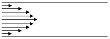
− A laminar flow is found when the velocities are relatively low. It is characterized by a distribution of velocities which are all parallel and whose profile is parabolic: the velocity of the fluid is maximum at the center and almost null when against the walls.

Figure 1.1. Profile of velocities in a laminar flow

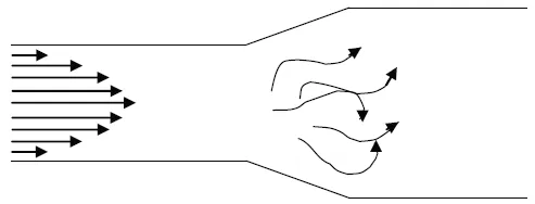
− A turbulent flow is a chaotic form of flow. The velocity then exhibits a vortical nature: local circular motions arise.

Figure 1.2. Profile of velocities in a turbulent flow

There are many reasons why a laminar flow could become a turbulent flow:

− the velocity of the flow surpasses a critical value;

− the structure of the vessels changes (see Figure 1.2).

Venous flow is laminar with a velocity that is constant overall.

Arterial flow is an intermediary case: it is laminar in diastole and turbulent during systole.

A turbulent flow causes significant artifacts in images of the flow, which we shall now go on to discuss in detail.

1.2. Basic phenomena in angiography

The flow phenomena which we are going to describe in this section enable us to spontaneously view blood vessels (without the injection of a contrast-enhancing product); the effect they have on the image depends on the sequence used (spin echo (SE) or gradient echo (GE)), on the parameters of that sequence (T_R, T_E…) but also on the particular parameters of the flow itself: its velocity, the orientation of the vessel in relation to the slice, etc.

Thus, we can construct a form of imaging relating to the flow: magnetic resonance angiography, or MRA.

1.2.1. Time of Flight (TOF)

When the vessel runs through the slice, the intensity of the flow signal depends on the time-of-flight of the protons T_t, i.e. the time taken to traverse the thickness ∆z of the plane being imaged at velocity V.

1.2.1.1. Phenomenon of flow void in a spin-echo sequence

We work on a spin-echo sequence where the 90° and 180° pulses are selective in the given slice.

With stationary protons: they experience both pulses and are therefore able to generate a signal.

With moving protons (in the bloodstream), two scenarios may arise:

– Either they remain in the slice (T_t < T_E/2) and are therefore struck by both pulses to generate a signal. For a vessel perpendicular to the slice, these protons have a velocity of V < ∆z/(T_E/2): this is qualified as a “slow” flow.

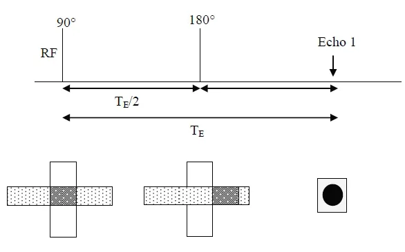
– Or they leave the slice entirely before the transmission of the 180° pulse (i.e. T_t < T_E/2). They are then replaced within the slice by protons which were not subjected to the initial 90° pulse and which therefore do not generate a signal. (The extreme case, T_t = T_E/2, is represented in Figure 1.3). For a vessel perpendicular to the slice, these protons have a velocity of V > ∆z/(T_E/2): this is qualified as a “fast” flow.

NOTE.– “Fast flow” is not necessarily synonymous with “arterial flow”: flow in large veins is also included in this category.

Figure 1.3. Case of T_t = T_E/2: the fate of protons experiencing the 90° excitation pulse (in white dots) and cross-sectional image of the flow

Flow void is the most commonly encountered phenomenon in flow imaging: this phenomenon accounts for the fact that many blood vessels are spontaneously visible on an MRI image by the absence of signal (by the “wall/light” contrast).

1.2.1.2. Phenomenon of flow-related (or paradoxical) enhancement

1.2.1.2.1 The phenomenon

We work on a spin-echo or gradient-echo sequence.

We suppose the T_R to be short: for this reason, there is repetition within a sufficiently short time period of the 90° excitation pulses.

With stationary protons: they have already been excited by the 90° pulse from the previous cycle (i.e. from the previous T_R interval): therefore, their longitudinal magnetization is low and they generate little signal.

With moving protons: if their velocity is sufficient, “fresh” protons, which have not been subjected to the 90° pulse from the previous cycle, enter into the slice: their longitudinal magnetization vector is maximum and the signal engendered by these protons is therefore maximum as well: this is the phenomenon of paradoxical enhancement.

1.2.1.2.2. The T_R dictates this phenomenon

The phenomenon of paradoxical enhancement is all the more marked when the TR is short: gradient-echo sequences (see below) are therefore more sensitive to this phenomenon, and therefore we shall limit ourselves to this type of sequence in our discussion below.

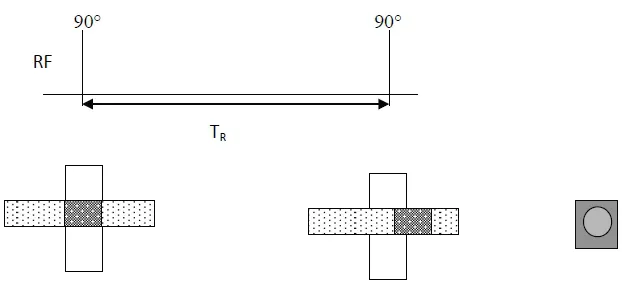
Figure 1.4. Case of T_t > T_R: fate of protons in the flow that experience the 90° excitation pulse (in white dots) and cross-sectional image of the flow. The vertical slab indicates all of the protons in the flow (in black dots) or outside of it (in white) affected by the different pulses

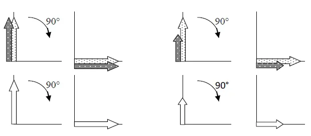
Figure 1.5. Case of T_t > T_R: longitudinal and transversal magnetization of the protons in the flow (top) and outside of it (bottom)

This phenomenon is maximum when all the protons excited during a cycle leave the slice and are replaced by “fresh” protons in the next cycle (T_t < T_R).

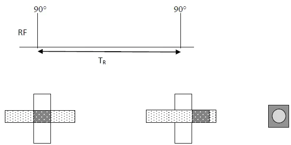
For a vessel running perpendicular to the slice, these protons have a velocity of V > ∆z/T_R. (The extreme case, with maximum contrast: T_t = T_R, is represented in Figure 1.6).

Figure 1.6. Case of T_t = T_R: fate of the protons in the flow that experience the 90° excitation pulse (in white dots) and cross-sectional image of the flow. The vertical strip indicates all the protons in the flow (in black dots) or outside of it (in white) affected by the different pulses

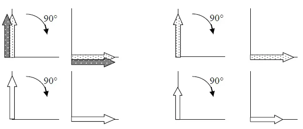
Figure 1.7. Case of T_t = T_R: longitudinal and transversal magnetization of the protons in the flow (top) and outside of it (bottom)

NOTE.– For spin-echo sequences, if T_R = 1s and ∆z = 1 cm, then paradoxical enhancement is maximum for velocities V > ∆z/T_R, i.e. V > 1 cm/s (this velocity, which is very slow, corresponds to venous flow at the end of diastole). The contrast obtained (the difference between flows of different velocities) is therefore very poor − all the more so if the stationary protons in the tissue are not saturated with a similarly long T_R.

This indeed reaffirms the necessity of working in a gradient-echo regime if we wish to use the paradoxical signal.

1.2.1.2.3. Single slice and multi-slice

In a multi-slice sequence, the paradoxical signal predominates over the first slice(s) (or the last) depending on the orientation of the flow (i.e. on the “flow entry slices”): such is the case for slice A in the diagram below.

Indeed, in planes which are a long way from the flow entry slices, the protons have been saturated by previous 90° excitations in the upstream slices (much like stationary protons): such is the case for slices C, D and E.

However, the paradoxical signal may also be visible on the first intermediary slices (slice B): sometimes we note the remnant presence of an intravascular “halo” signal in these slices. This halo is due to the differences in velocity of the protons at the center of the vessel (fast flow) and at the edges of the vessel (slow flow) in the case of a laminar flow with parabolic profile.

Figure 1.8. Paradoxical enhancement in a multi-slice sequence

NOTE.– The gradient-echo sequence, which is favored when we wish to use the paradoxical signal, usually enables us to take ver...

Table of contents

• Cover
• Contents
• Title Page
• Copyright
• Chapter 1: Flow
• Chapter 2: Diffusion
• Chapter 3: Perfusion
• Chapter 4: Functional MRI
• Bibliography
• Index