Microfluidics

Stéphane Colin, Stéphane Colin

• Publisher: Wiley-ISTE
• Year: 2013
• ISBN:
  9781118599884
• Edition: 1
• Topic: Technology & Engineering
• Subtopic: Microelectronics
• Index: Technology & Engineering

The recent development of microscale technologies makes it possible to design complex microsystems devoted to transport, dosing, mixing, analysis or even synthesis of fluids. Applications are numerous and exist in almost every industrial field, from biotechnology and healthcare to aeronautics and advanced materials manufacturing. Microfluidics is a relatively new research area, usually comprising work with microsystems and involving internal fluid flows with characteristic dimensions of the order of one micrometer (1 x 10 -6 m).

This book provides engineers and researchers with a range of tools for modeling, experimenting on, and simulating these microflows, as a preliminary step in designing and optimizing fluidic microsystems. The various consequences of miniaturization on the hydrodynamics of gas, liquid or two-phase flows, as well as on associated heat transfer phenonema, are analyzed.

The book is illustrated with examples that demonstrate the wide diversity of applications, and the breadth of novel uses of these fluidic microsystems.

Chapter 1

Introduction to Microflows ¹

1.1. Fluid mechanics, fluidics and microfluidics

From the first aqueducts to modern oil extraction networks, man has always been confronted with handling fluids, the transport of which he has tried to control and optimize. For 2,000 years, from Archimedes (in 300 BC) and Torricelli and Pascal in the 17^th Century, to da Vinci in the 15^th Century, knowledge only concerned fluids at rest. Flow modeling really started and expanded once Isaac Newton was able to concisely write his three famous laws of motion. After this, the foundations of hydrodynamics were laid in the 18^th Century by d’Alembert, Euler and Bernoulli, and the physics of complex flows fully developed in the 19^th Century, notably with the works of Navier, Stokes, Couette and Reynolds.

Among these illustrious researchers, we can cite French physiologist Jean-Louis Marie Poiseuille, a talented experimenter who was interested in blood circulation and studied the flow of viscous fluids through capillary tubes. In 1840, he succeeded in measuring flowrates in glass capillaries around 10 µm in diameter [POI 40] and he showed that the classic laws of flow were still applicable at such a small scale. Thus, he can be considered a pioneer in microfluidics.

The word microfluidics, however, has only appeared recently, in the early 1980s, although microflows have interested a growing scientific community in the field of blood microcirculation (see Chapter 4), flows in porous media and lubrication for a long time. Its older relative, fluidics, was in fashion in the 1960s and 1970s. Fluidics seems to have started in the USSR in 1958 and then developed in the US and Europe; first for military purposes, with civil applications appearing later. At that time, fluidics was mainly concerned with inner gas flows in devices involving millimetric or sub-millimetric sizes. These devices were designed to perform the same actions (amplification, logic operations, diode effects, etc.) as their electric counterparts. The idea was to design pneumatically, rather than electrically, supplied computers. The main applications were in the spatial domain, for which electric power overload was an issue due to the electric components of the time that generated excessive magnetic fields and dissipated too much thermal energy to be safe in a confined space. Most of the fluidic devices were etched in a substrate by means of conventional machining techniques or by insolation techniques applied on specific resins, where masks protected the parts that needed to be preserved.

Figure 1.1. Some examples of fluidic elements: a: jet deflection amplifier; b) fluidic oscillator (adapted from [AND 67]); and c) temperature sensor (adapted from [HAL 67])

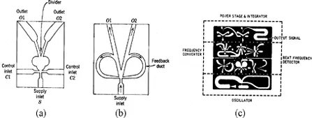
The rapid development of microelectronics put a sudden end to pneumatic computers, but the last two decades have seen a particular enhancement of our knowledge about the design of complex fluidic elements, such as diodes, amplifiers or oscillators (see Figure 1.1).

Microsystems emerged in the 1980’s and microfluidics appeared at the same time. Microfluidics relates to flows inside devices with inner sizes in the order of 1 µm. As was the case for fluidics, the main findings about microfluidic systems first concerned technological breakthroughs: adaptation of microfabrication techniques and elaboration of new concepts. The need for experiments and modeling in fluid mechanics arrived later and today involves a broad scientific community in America, Asia and Europe.

Following the first idea launched by Physics Nobel Prize winner Richard Feynman to exploit capabilities of micro- and nanotechnologies for mechanical purposes¹, things have considerably progressed, especially over the past 20 years. One main goal of MEMS (micro-electro-mechanical systems) with their millimetric external and micrometric internal dimensions was to do things better, quicker and above all cheaper.

Thus, the global markets² and forecasts for the MEMS supply chain, including MEMS systems, devices, equipment and materials, was €705 billion ($960 billion) in 2007 and is estimated to reach €1,400 billion ($1, 910 billion) in 2012! A number of these microsystems use or transport fluids; some of them are designed for elementary operations, such as fluid transport or dosing, but others have to achieve much more complex functions, such as flow mixing, analysis or even synthesis. There are a great number of applications that concern various fields (see section 1.5).

The question for us is what is the impact of high-level miniaturization on the behavior of internal flows? Obviously, the decrease in scale does not just involve a homothety, and for several reasons the behavior of fluidic microsystems cannot be directly deduced from one of the usual hydraulic or pneumatic systems, using a simple law of proportionality. The first reason is that, the shape of microsystems is generally very different to what we know for classical sizes (see Chapter 8); fabrication techniques also being very different (see section 1.4). Second, flows depend on a series of parameters and most of them are not simply proportional to a characteristic length. Last, some assumptions that are fully justified in classic fluid mechanics are no longer valid at the scale of microflows.

1.2. Scaling effects and microeffects

A scaling effect can be analyzed through the dependence of various mechanical variables X vis-à-vis a characteristic length L of the flow [TRI 02, ZOH 03]. It does not necessarily introduce new physical laws or mechanisms but takes part in a redistribution of dominating effects. Some examples illustrate this dependence in Table 1.1, in the form:

[1.1]

assuming that the density ρ does not depend on the characteristic length, which reads:

[1.2]

Table 1.1. Effect of length scale decrease on some mechanical variables

Considering two variables X₁ and X₂ of the same type, if

(X₁) <

(X₂), the decrease of the characteristic length L will increase the importance of X₁ vis-à-vis X₂. The accelerations a should be considered as consequences of forces (a = F/m) and as such, their dependence vis-à-vis L can be directly deduced:

[1.3]

Thus, even if time does not depend on L, the response time

of a system depends on it via the accelerations – and consequently the forces – at work:

[1.4]

Finally, the power per volume unit

also has dependence in the form:

[1.5]

1.2.1. Importance of surface effects

The increase of the area A over volume V ratio leads to various consequences. In balance equations, it gives a dominating weight to mass, momentum or energy fluxes compared with storage and generation terms. This leads to very different physical behaviors, as illustrated by the following experiment which consists of letting an ice cube...

Table of contents

• Cover
• Title Page
• Copyright
• Preface
• Chapter 1: Introduction to Microflows
• Chapter 2: Gaseous Microflows
• Chapter 3: Liquid Microflows: Particularities and Modeling
• Chapter 4: Physiological Microflows
• Chapter 5: Single-phase Heat Transfer
• Chapter 6: Two-Phase Microflows
• Chapter 7: Experimental Methods
• Chapter 8: Fluidic Microsystems
• Chapter 9: Microsystems in Macroflows Active Control
• List of Authors
• Index