A Quantitative Approach to Commercial Damages

Applying Statistics to the Measurement of Lost Profits

Mark G. Filler, James A. DiGabriele

• Publisher: Wiley
• Year: 2012
• ISBN:
  9781118236376
• Edition: 1
• Topic: Business
• Subtopic: Accounting
• Index: Business

How-to guidance for measuring lost profits due to business interruption damages

A Quantitative Approach to Commercial Damages explains the complicated process of measuring business interruption damages, whether they are losses are from natural or man-made disasters, or whether the performance of one company adversely affects the performance of another. Using a methodology built around case studies integrated with solution tools, this book is presented step by step from the analysis damages perspective to aid in preparing a damage claim. Over 250 screen shots are included and key cell formulas that show how to construct a formula and lay it out on the spreadsheet.

• Includes Excel spreadsheet applications and key cell formulas for those who wish to construct their own spreadsheets
• Offers a step-by-step approach to computing damages using case studies and over 250 screen shots

Often in the course of business, a firm will be damaged by the actions of another individual or company, such as a fire that shuts down a restaurant for two months. Often, this results in the filing of a business interruption claim. Discover how to measure business losses with the proven guidance found in A Quantitative Approach to Commercial Damages.

CHAPTER 1

Case Study 1—Uses of the Standard Deviation

In this and all the other case studies in this book, you will come across statistical terms that will be unfamiliar to you. Rather than explain each term in the body of the case study, or populate each case study with explanatory foot- or endnotes, we have provided a glossary at the end of the book to facilitate your understanding of the text.

The Steps of Data Analysis

An important step in data analysis, and hence forecasting, is to determine the shape, center, and spread of your data set. That is, how are the data distributed (normally, uniformly, or left- or right-skewed), what is its mean and median, and to what degree is it dispersed about the mean? The answers to these questions are important, as they will determine what statistical tools we can use as we attempt to determine lost profits. The questions can be answered graphically with histograms, stem and leaf plots, and box plots as well as computationally through the use of various Excel descriptive statistical functions such as AVERAGE, STDEVP, SKEW, and KURT. Knowing a data set's distribution (normal, or at least near–bell shaped), its center (mean), and its spread (standard deviation), we can begin to draw conclusions about it that will allow us to meaningfully compare it with other contemporaneous data points.

Our first case, while not strictly on the subject of lost profits, is about an issue our readers see all the time in their practices. The case concerns the value of a business on June 30, 2010, for shareholder buyout purposes. The subject company's year-to-date (YTD) gross margin of 14.4 percent at the June 30 date of loss was substantially below its nine-year historical average. We want to know if this difference is statistically significant and if so, what the probability of its occurrence is. In order to run the tests to help answer these questions, we need to assure ourselves that the distribution of the nine years'1 gross margins is, if not normal in shape, at least near–bell shaped. We begin this process with the following calculations and charts.

Shape

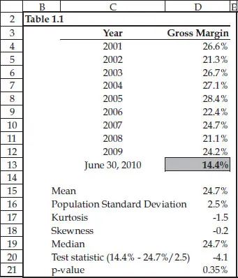
As shown in Table 1.1, the nine-year average gross margin is 24.7 percent; its standard deviation is 2.5 percent (we are treating the nine years as the population, not a sample, so the Excel function is STDEVP); it is symmetrical,2 as its median of 24.7 percent equals its mean; and it is near–bell shaped, as both KURT and SKEW return results that are between –1.5 and +1.5. While there are too few data points to construct a meaningful histogram to informally test for normality, we can create a normal P-plot, or probability plot, where we match up our nine observations with the normal scores that we would expect to see if the data came from a standard normal distribution. If our nine observations follow a general straight line on the normal probability plot, especially at both ends, we can feel assured that the data are near–bell shaped.

Table 1.1

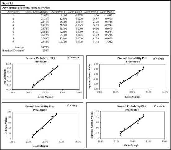
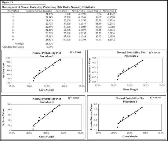
Figure 1.1 demonstrates four methods for producing the expected values for a P-plot, with no one method being superior to the others. The reader can choose any one method he or she prefers. Since two of the methods require that the data be ranked, we first sorted the gross margins from smallest to largest, and then applied the particular formula for each method and charted the results.

Figure 1.1

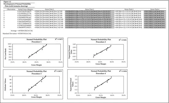
For ease of understanding, we have also shown the formulas for each method in Figure 1.2. But a nagging question remains: If all the observations do not lie directly on the trendline, how do we know that the data are still near–bellshaped? The answer to that question is shown in Figure 1.3, where we have substituted nine numbers created by using Excel's random number generator, which is found in the Analysis ToolPak. Selecting normal distribution from the analysis tool's drop-down menu, and then filling in the rest of the dialogue box with the mean and standard deviation of the original nine observations, produces nine random numbers that are normally distributed with approximately the same mean and standard deviation as the original nine gross margin numbers.

Figure 1.2

Comparing the two sets of charts in Figure 1.1 and Figure 1.3, we can see that both data sets have the same degree of deviation about the trendline, indicating that the original data set can be considered near–bell shaped. This near–bell shape of the distribution allows us to use parametric tests that involve the use of the two parameters of the distribution, its mean and standard deviation. Absent this shape, we would have to turn to nonparametric methods, a subject we leave to another book.

Figure 1.3

Spread

The next step is to create a test statistic that measures how far June 30's 14.4 percent is from the nine-year average gross margin. The test statistic is: (X – mean)/standard deviation, or (14.4 – 24.7)/2.5. The resulting statistic, called a z-score, of –4.1 indicates that 14.4 percent is 4.1 standard deviations below the nine-year average. Is this too far from the average for our purposes? We know from the empirical rule that if a data set is near–bell shaped, then approximately 95 percent of its observations will fall within ±2 standard deviations from the mean, and 99.7 percent of its observations will fall within ±3 standard deviations from the mean. At 4.1 standard deviations below average, June 30's gross margin is literally off the charts. In fact, using Excel's NORMDIST function, we can show that there is only a 0.35 percent chance that the gross margin on June 30 of 14.4 percent was drawn from the same pool as the nine year-end gross margins.

Once this, and its implication that they were deliberately cooking the books to lower the value of the company, was pointed out to the other side, they immediately increased their buyout offer by 50 percent.

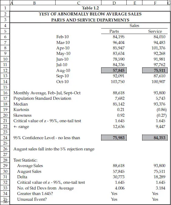
Our second situation involves a car dealership that experienced a small fire in its parts department in early August 2010, and then claimed lost sales for weeks afterwards. Are the decreases in parts and service departmental sales during the month of August 2010 greater than 1.645 or more standard deviations of the historical average, and therefore statistically significant, or are the decreases in the normal course of business? Our procedure is essentially the same as that just described in the first situation. We begin by analyzing the previous six and succeeding two months of sales and find that both data sets are near–bell shaped—the median approximates the mean, and kurtosis and skewness measures are between –1.5 and +1.5 as shown in Table 1.2. Unlike situation 1, where the question posed was whether June 30's sales were different in either direction, that is, greater or lesser, from the nine-year average, in situation 2 we only want to know if August's sales are less than the average—statistically speaking, situation 1 called for a two-tailed test and situation 2 calls for a one-tailed test.

Table 1.2

The cutoff point for a one-tailed test is 1.645 standard deviations if we are willing to be wrong about our conclusions 5 percent of the time. That is, we enter the 5 percent rejection area at 1.645 standard deviations, rather than the 1.96 standard deviations of a two-tailed test. Multiplying the population standard deviation by 1.645 and subtracting the product from the eight-month average sales for both departments gives us the lower limit of our 95 percent confidence level. For example, in the parts department, average sales equaled $88,618, and the standard deviation was $7,682. Multiplying $7,682 by 1.645 gives us $12,636. Subtracting this from average sales gives us $75,983, an amount greater than August's sales of $57,845. Since actual sales for August are less than $75,983, we can say with 95 percent confidence that those sales did not decrease in the ordinary course of business—that there was some intervention that caused them to be this far below average. As such, after subtracting avoided costs, the insured's claim for lost profits was honored.

Conclusion

In this chapter we demonstrated how the standard deviation can be applied in situations where the data set you are working with is the population, and not a sample. How does one know whether the data set is a sample or a population? The answer lies in whether or not you make inferences outside the data set. For example, a classroom of 30 students is a population if all your statistical tests and inferences are about the 30 students. But if you are going to use the statistical test results of those 30 students to make inferences about other students in other classrooms, then you are working with a sample.

In the next chapter we introduce you to various data analysis techniques that should precede any selection of a sales forecasting methodology.

Notes

1. Generally speaking, in statistics, the larger the sample size, the better the results. However, in damages cases, the analyst has to work with what is given. Therefore, while for academic research a sample size of 9 would probably be considered too small, for litigation purposes it will have to do.

2. If folded over at the midpoint, its left side would be a mirror image of its right side.

CHAPTER 2

Case Study 2—Trend and Seasonality Analysis

May 31, 2010, was a dark and stor...

Table of contents

• Cover
• Series
• Title Page
• Copyright
• Dedication
• Preface
• Acknowledgments
• INTRODUCTION: The Application of Statistics to the Measurement of Damages for Lost Profits
• CHAPTER 1: Case Study 1—Uses of the Standard Deviation
• CHAPTER 2: Case Study 2—Trend and Seasonality Analysis
• CHAPTER 3: Case Study 3—An Introduction to Regression Analysis and Its Application to the Measurement of Economic Damages
• CHAPTER 4: Case Study 4—Choosing a Sales Forecasting Model: A Trial and Error Process
• CHAPTER 5: Case Study 5—Time Series Analysis with Seasonal Adjustment
• CHAPTER 6: Case Study 6—Cross-Sectional Regression Combined with Seasonal Indexes to Determine Lost Profits
• CHAPTER 7: Case Study 7—Measuring Differences in Pre- and Postincident Sales Using Two Sample t-Tests versus Regression Models
• CHAPTER 8: Case Study 8—Interrupted Time Series Analysis, Holdback Forecasting, and Variable Transformation
• CHAPTER 9: Case Study 9—An Exercise in Cost Estimation to Determine Saved Expenses
• CHAPTER 10: Case Study 10—Saved Expenses, Bivariate Model Inadequacy, and Multiple Regression Models
• CHAPTER 11: Case Study 11—Analysis of and Modification to Opposing Experts' Reports
• CHAPTER 12: Case Study 12—Further Considerations in the Determination of Lost Profits
• CHAPTER 13: Case Study 13—A Simple Approach to Forecasting Sales
• CHAPTER 14: Case Study 14—Data Analysis Tools for Forecasting Sales
• CHAPTER 15: Case Study 15—Determining Lost Sales with Stationary Time Series Data
• CHAPTER 16: Case Study 16—Determining Lost Sales Using Nonregression Trend Models
• APPENDIX: The Next Frontier in the Application of Statistics
• Bibliography of Suggested Statistics Textbooks
• Glossary of Statistical Terms
• About the Authors
• Index