Rasch Models in Health

Karl Bang Christensen, Svend Kreiner, Mounir Mesbah

• Publisher: Wiley-ISTE
• Year: 2013
• ISBN:
  9781118574546
• Edition: 1
• Topic: Mathematics
• Subtopic: Applied Mathematics
• Index: Mathematics

The family of statistical models known as Rasch models started with a simple model for responses to questions in educational tests presented together with a number of related models that the Danish mathematician Georg Rasch referred to as models for measurement. Since the beginning of the 1950s the use of Rasch models has grown and has spread from education to the measurement of health status. This book contains a comprehensive overview of the statistical theory of Rasch models.

Part 1 contains the probabilistic definition of Rasch models, Part 2 describes the estimation of item and person parameters, Part 3 concerns the assessment of the data-model fit of Rasch models, Part 4 contains applications of Rasch models, Part 5 discusses how to develop health-related instruments for Rasch models, and Part 6 describes how to perform Rasch analysis and document results.

PART 1

Probabilistic Models

Introduction

This part introduces the models that are analyzed in the book. The Rasch model was originally formulated by Georg Rasch for dichotomous items [RAS 60]. This model is described in Chapter 1, where different parameterizations are also introduced. The sources of polytomous Rasch models are less clear. Georg Rasch formulated a quite general polytomous model where each item measures several latent variables [RAS 61]. However, this model has seen little use. Later, several authors [AND 77, AND 78, MAS 82] formulated models where items with more than two response categories measure a single underlying latent variable.

Bibliography

[AND 77] ANDERSEN E.B., “Sufficient statistics and latent trait models”, Psychometrika, vol. 42, pp. 69–81, 1977.

[AND 78] ANDRICH D., “A rating formulation for ordered response categories”, Psychometrika, vol. 43, pp. 561–573, 1978.

[MAS 82] MASTERS G.N., “A Rasch model for partial credit scoring”, Psychometrika, vol. 47, pp. 149–174, 1982.

[RAS 60] RASCH G., Probabilistic Models for Some Intelligence and Attainment Tests, Danish National Institute for Educational Research, Copenhagen, 1960.

[RAS 61] RASCH G., “On general laws and the meaning of measurement in psychology”, Proceedings of the Fourth Berkeley Symposium on Mathematical Statistics and Probability, IV, University of California Press, Berkeley, CA, pp. 321–334, 1961.

Chapter 1

The Rasch Model for Dichotomous Items

1.1. Introduction

The family of statistical models, which is known as Rasch models, was first introduced with a simple model for responses to dichotomous items (questions) in educational tests [RAS 60]. It was presented together with a number of related models that the Danish mathematician Georg Rasch called models for measurement. Since then, the family of Rasch models has grown to encompass a number of statistical models.

1.1.1. Original formulation of the model

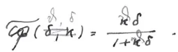
All Rasch models share a number of fundamental properties, and we introduce this book with a brief recapitulation of the very first Rasch model: the Rasch model for dichotomous items. This model was developed during the 1950s when Georg Rasch got involved in educational research. The model describes responses to a number of items by a number of persons assuming that responses are stochastically independent, depending on unknown items and person parameters. In Rasch’s original conception of the model (see Figure 1.1), the structure of the model was multiplicative. In this model, the probability of a positive response to an item depends on a person parameter ξ and an item parameter δ in such a way that the probability of a positive response to an item depends on the product of the person parameter and the item parameter.

Figure 1.1. The Rasch model 1952/1953

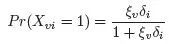
If we refer to the response of person v to item i as X_vi and code a positive response as 1 and a negative response as 0, the Rasch model asserts that

[1.1]

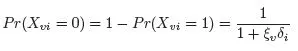
where both parameters are non-negative real numbers. It follows from [1.1] that

[1.2]

The interpretation of the parameters in this model is straightforward: the probability of a positive response increases as the parameters increase toward infinity. In educational testing, the person parameter represents the ability of the student and the item parameter represents the easiness of the item: the better the ability and the easier the item, the larger the probability of a correct response to the item. In health sciences, the person parameter could represent the level of depression whereas the item parameters could represent the risk of experiencing certain symptoms relating to depression.

EXAMPLE 1.1.– Consider the following dichotomous items intended to measure depression:

1) Did you have sleep disturbance every day for a period of two weeks or more?

2) Did you have a loss or decrease in activities every day for a period of two weeks or more?

3) Did you have low self-esteem every day for a period of two weeks or more?

4) Did you have decreased appetite every day for a period of two weeks or more?

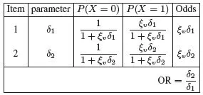
Items like these appear in several questionnaires. According to the Rasch model, responses to these items depend on the level of depression measured by the ξ parameter and on four item parameters δ₁–δ₄. In a recent study, the item parameters were found to be 2.57, 1.57, 0.52 and 0.48, respectively [FRE 09, MES 09]. The interpretation of these numbers is that sleep disturbance is the most common and loss of appetite is the least common of the four symptoms. To better understand the role of the item parameters, we have to look at the relationships between the probabilities of positive responses to two questions. This is shown in Table 1.1, where it can be seen that the ratio between the two item parameters is the odds ratio (OR) comparing the odds of encountering the symptoms described by the items irrespective of the level of depression ξ of the persons. This interpretation should be familiar to persons with a working knowledge of epidemiological methods. According to the Rasch model, the level of depression does not modify the relative risk of the symptoms. In the theory of Rasch models, this is sometimes called no item-trait interaction.

Table 1.1. Response probabilities for two items when the person parameter is ξ_v

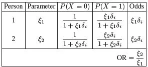
EXAMPLE 1.2.– Since the item parameters for the first two items are 2.57 and 1.57, we see that the odds ratio relating the risk of loss of or reduction of activities to the risk of sleep disturbances is equal to 1.57/2.57 = 0.613. Because of the symmetry in formula [1.1] the same argument applies to comparisons of persons. Table 1.2 considers the risk of encountering a specific symptom for each of two persons with different levels of depression. As for the items, we interpret the ratio between the person parameters as the odds ratio comparing the risk for person two to the risk for person one.

Table 1.2. Response probabilities for an item with an item parameter equal to δ_i

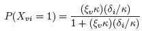
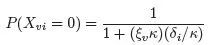
To measure the level of depression, we have to estimate the parameter ξ based on observed item responses. However, this parameter is not identifiable in absolute terms because the probabilities [1.1] depend on the product of the person and item parameters. Multiplying all person parameters by a constant к and dividing all item parameters by the same constant results in a reparameterized model

[1.3]

[1.4]

with exactly the same formal structure and the same probabilities as the original model, and where the odds ratio comparing response probabilities for the two persons is the same as in Table 1.2. To identify the parameters, we consequently have to impose restrictions on the parameters. The standard way of doing this is to fix the parameters such that the product of the item parameters is equal to one. The parameters of the depression items above were fixed in this way. Another way that may be more natural for an epidemiologist would be to select a reference item where the item parameter is equal to one. The item parameters for other items are then interpretable as ORs comparing the item to the reference item (see Table 1.1). Because of the symmetry in formula [1.1], similar arguments ...

Table of contents

• Cover
• Table of Contents
• Title page
• Copyright page
• Preface
• PART 1: Probabilistic Models
• PART 2: Inference in the Rasch Model
• PART 3: Checking the Rasch Model
• PART 4: Applying the Rasch Model
• PART 5: Creating, Translating and Improving Rasch Scales
• PART 6: Analyzing and Reporting Rasch Models
• List of Authors
• Index