Full-Field Measurements and Identification in Solid Mechanics

Michel Grediac, Francois Hild, Michel Grediac, Francois Hild

• Publisher: Wiley-ISTE
• Year: 2012
• ISBN:
  9781118578476
• Edition: 1
• Topic: Physical Sciences
• Subtopic: Mechanics

This timely book presents cutting-edge developments by experts in the field on the rapidly developing and scientifically challenging area of full-field measurement techniques used in solid mechanics – including photoelasticity, grid methods, deflectometry, holography, speckle interferometry and digital image correlation. The evaluation of strains and the use of the measurements in subsequent parameter identification techniques to determine material properties are also presented.

Since parametric identification techniques require a close coupling of theoretical models and experimental measurements, the book focuses on specific modeling approaches that include finite element model updating, the equilibrium gap method, constitutive equation gap method, virtual field method and reciprocity gap method. In the latter part of the book, the authors discuss two particular applications of selected methods that are of special interest to many investigators: the analysis of localized phenomenon and connections between microstructure and constitutive laws. The final chapter highlights infrared measurements and their use in the mechanics of materials.

Written and edited by knowledgeable scientists, experts in their fields, this book will be a valuable resource for all students, faculties and scientists seeking to expand their understanding of an important, growing research area

Chapter 1

Basics of Metrology and Introduction to Techniques

Chapter written by André CHRYSOCHOOS and Yves SURREL.

1.1. Introduction

Full-field optical methods for kinematic field measurement have developed tremendously in the last two decades due to the evolution of image acquisition and processing. Infrared (IR) thermography has also dramatically improved due to the extraordinary development of IR cameras. Because of their contactless nature, the amount of information they provide, their speed and resolution, these methods have enormous potential both for the research lab in the mechanics of materials and structures and for real applications in industry.

As for any measurement, it is essential to assess the obtained result. This is the area of metrology. The ultimate goal is to provide the user with as much information as possible about the measurement quality. We deal with a specific difficulty for the quality assessment of the optical methods that arises precisely from their full-field nature. The metrology community is far more familiar with point-wise or average scalar measurements (length, temperature, voltage, etc.). Currently, the metrology of full-field optical methods is not yet fully settled. However, the wide dissemination of these techniques will only efficiently occur when users have a clear understanding of how they can characterize the measurement performances of the equipment that vendors put on the market.

First, the goal of this chapter is to present some basic elements and concepts of metrology. It is by no means exhaustive, and only aims at presenting the basics of the domain in a simple way, so that the researchers, users, developers and vendors can exchange information based on well-established concepts. Second, we will rapidly present the different optical techniques based on their main characteristics (how information is encoded, interferential or not, etc.).

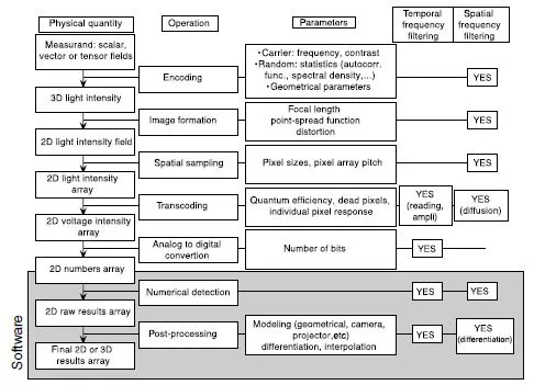
It should be noted that optical measurement techniques exhibit a non-negligible amount of complexity. Figure 1.1 outlines the typical structure of a measurement chain that leads from a physical field to a numerical measurement field using a camera. It can be seen that there are many steps required to obtain the final result that the user is interested in, and numerous parameters that may impair the result and effects are involved at each step. Most importantly, there are usually numerical postprocessing stages that are often “black boxes” whose metrological characteristics or impact may be difficult or even impossible to obtain from the supplier of the equipment in the case of commercial systems.

Figure 1.1. Outline of the many steps involved in a measurement chain using a camera

1.2. Terminology: international vocabulary of metrology

1.2.1. Absolute or differential measurement

In any scientific domain, terminology is essential. Rather than enumerating the main terms to use (precision, sensitivity, resolution, etc.), let us try to adopt the final user point of view. What are the questions he generally asks, and in which context? There are, in fact, not so many questions, and each of them leads naturally to the relevant metrological term(s):

1) Is the obtained result “true”, “exact” and “close to reality”? How to be confident in the result?

2) Is the equipment “sensitive”? Does it see small things?

These two questions lie behind the separation of metrology into two distinct domains, within which the metrological approach will be different: absolute measurement and differential measurement.

1.2.1.1. Absolute measurement

Here, we seek the “true” value of the measurand (the physical quantity to measure), for example to assess that the functional specifications of a product or system are met. Dimensional metrology is an obvious example. The functional quality of a mechanical part will most often depend on the strict respect of dimensional specifications (e.g. diameters in a cylinder/piston system). The user is interested in the deviation between the obtained measurement result and the true value (the first of the two questions above). This deviation is called the measurement error. This error is impossible to know, and here is where metrology comes in. The approach used by metrologists is a statistical one. It will consist of evaluating the statistical distribution of the possible errors, and characterizing this distribution by its width, which will represent the average (typical) deviation between the measurement and the true value. We generally arrive here at the concept of measurement uncertainty, which gives the user information about the amount of error that is likely to occur.

It is worth mentioning that some decades ago, the approach was to evaluate a maximum possible deviation between the measurement and the real value. The obtained uncertainty values were irrelevantly overestimated because the uncertainty was obtained by considering that all possible errors were synergetically additive in an unfavorable way. Today, we take into account that statistically independent errors tend to average each other out to a certain extent. In other words, it is unlikely (and this is numerically evaluated) that they act coherently together to impair the result in the same direction. This explains the discrepancy between the uncertainty evaluation formulas that can be found in older treatises and those used today. As an example, if c = a + b, where a and b are independent measurements having uncertainties Δa and Δb, the older approach (maximum upper bound) would yield Δc = Δa + Δb, but the more recent approach gives

, these two values being in a non-negligible ratio of

= 1.414 in the case Δa, = Δb.

1.2.1.2. Differential measurement

Now, let us consider that the user is more interested in the deviation from a “reference” measurement. In the mechanics of materials field, the reference measurement will most likely be the measurement in some initial state, typically before loading. It is basically interesting to perform measurements in a differential way, and this is done for two reasons:

– As the measurement conditions are often very similar, most systematic errors will compensate each other when subtracting measurement results to obtain the deviation; typically, optical distortion (image deformation) caused by geometrical aberrations of the camera lens will be eliminated in a differential measurement.

– Measurement uncertainty is only about the difference, which implies that interesting results can be obtained even with a system of poor quality; let us take an example of a displacement measurement system exhibiting a systematic 10% error. Absolute measurements obtained with this system would probably be considered unacceptable. However, when performing differential measurements, this 10% error only affects the difference between the reference and actual measurements. Consider the following numerical illustration: with a first displacement of 100 μm and a second displacement of 110 μm; this hypothetical system would provide measured values of 90 and 99 μm, roughly a 10 μm error each time, probably not acceptable in an absolute positioning application, for example. But the measurement differential displacement is 9 μm, which is only a 1 μm error.

Regarding this second example, we should emphasize the fact that it is not possible to use relative uncertainty (percentage of error) with differential measurements because this relative uncertainty, ratio between the uncertainty and the measurand, is related to a very small value, the difference of measurements, that is nominally zero. Hence, “percentage of error” is strictly meaningless in the case of differential measurements. Only absolute uncertainty is meaningful in this case.

1.2.2. Main concepts

We will consider in this section the main concepts of metrology. The corresponding terms are standardized in a document (International Vocabulary of Metrology, abbreviated as “VIM”, [VIM 12]) which can be downloaded freely from the BIPM website.

1.2.2.1. Measurement uncertainty

The VIM definition is as follows:

non-negative parameter characterizing the dispersion of the quantity values being attributed to a measurand, based on the information used.

The underlying idea is that the measurement result is a random variable, which is characterized by a probability density function centered at a certain statistical average value. This probability density function is typically bell-shaped. Note # 2 in the VIM states:

the parameter may be, ...

Table of contents

• Cover
• Contents
• Title page
• Copyright page
• Foreword
• Introduction
• Chapter 1: Basics of Metrology and Introduction to Techniques
• Chapter 2: Photoelasticity
• Chapter 3: Grid Method, Moiré and Deflectometry
• Chapter 4: Digital Holography Methods
• Chapter 5: Elementary Speckle Interferometry
• Chapter 6: Digital Image Correlation
• Chapter 7: From Displacement to Strain
• Chapter 8: Introduction to Identification Methods
• Chapter 9: Parameter Identification from Mechanical Field Measurements using Finite Element Model Updating Strategies
• Chapter 10: Constitutive Equation Gap
• Chapter 11: The Virtual Fields Method
• Chapter 12: Equilibrium Gap Method
• Chapter 13: Reciprocity Gap Method
• Chapter 14: Characterization of Localized Phenomena
• Chapter 15: From Microstructure to Constitutive Laws
• Chapter 16: Thermographic Analysis of Material Behavior
• List of Authors
• Index