Arbitrary Lagrangian Eulerian and Fluid-Structure Interaction

Numerical Simulation

M'hamed Souli, David J. Benson

• Publisher: Wiley-ISTE
• Year: 2013
• ISBN:
  9781118618684
• Edition: 1
• Topic: Tecnología e ingeniería
• Subtopic: Ingeniería civil

This book provides the fundamental basics for solving fluid structure interaction problems, and describes different algorithms and numerical methods used to solve problems where fluid and structure can be weakly or strongly coupled.

These approaches are illustrated with examples arising from industrial or academic applications. Each of these approaches has its own performance and limitations. The added mass technique is described first. Following this, for general coupling problems involving large deformation of the structure, the Navier-Stokes equations need to be solved in a moving mesh using an ALE formulation. The main aspects of the fluid structure coupling are then developed. The first and by far simplest coupling method is explicit partitioned coupling. In order to preserve the flexibility and modularity that are inherent in the partitioned coupling, we also describe the implicit partitioned coupling using an iterative process. In order to reduce computational time for large-scale problems, an introduction to the Proper Orthogonal Decomposition (POD) technique applied to FSI problems is also presented. To extend the application of coupling problems, mathematical descriptions and numerical simulations of multiphase problems using level set techniques for interface tracking are presented and illustrated using specific coupling problems.

Given the book's comprehensive coverage, engineers, graduate students and researchers involved in the simulation of practical fluid structure interaction problems will find this book extremely useful.

Chapter 1

Introduction to Arbitrary Lagrangian–Eulerian in Finite Element Methods ¹

1.1. Introduction

The choice of the coordinate system for the numerical solution of a partial differential equation is both the first and arguably the most important decision. An inappropriate choice will lead to a numerical method that is both expensive and inaccurate. Traditionally, problems in structural engineering and solid mechanics have used a Lagrangian coordinate system, with the computational mesh moving with the material. This choice is very economical and resolves the material boundaries very accurately. Its primary limitation is that the deformations must be limited otherwise the distortion in the mesh will result in inaccuracies and numerical instability. The traditional choice for fluid mechanics is a Eulerian coordinate system having the mesh fixed in space. Using a fixed mesh eliminates the limitation on the degree of deformation permitted in the material, but introduces the additional complexity of the convective terms associated with the transport of the material through the mesh.

For problems with both fluids and solids, such as fluid– structure interaction, neither the Lagrangian nor the Eulerian formulations are optimal for the entire domain. A Lagrangian formulation cannot handle the large deformations of the fluid and a Eulerian formulation sacrifices some accuracy when applied to solids. Most fluid–structure interaction formulations use a Eulerian formulation for the fluid and a Lagrangian formulation for the structure, and introduce a coupling algorithm between them. The coupling algorithm is quite complex if it is required to handle an arbitrary Lagrangian mesh overlapping a Eulerian mesh. It can be simplified to a larger extent if the boundary of the fluid mesh conforms to the boundary of the Lagrangian mesh, and the nodes of both meshes are superposed along their common boundary.

Arbitrary Lagrangian–Eulerian (ALE) methods allow the mesh to move in an arbitrary manner, with the two limiting cases reducing to the Lagrangian and Eulerian formulations. An ALE mesh that conforms to the Lagrangian mesh for the structure along part of its boundary while the rest remains fixed providing a convenient transition between the fluid and the structure. Since the ALE mesh moves relative to the material, it has transport terms similar to those found in the Eulerian formulation, and therefore it has many algorithms in common with computational fluid dynamics (CFD).

This chapter provides an introduction to the basic ideas behind the ALE formulation with an emphasis on methods appropriate for problems in solid mechanics and introduces some of the numerical methods most commonly used in ALE calculations to solve them.

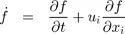
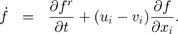
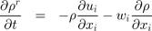
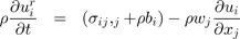
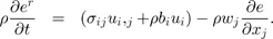
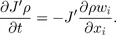
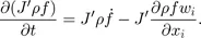
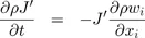
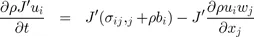
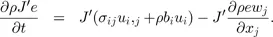
1.2. Governing equations

In this section, the governing equations are derived for the case when the reference coordinates move at an arbitrary velocity [NOH 64, HUG 81, DON 83]. This formulation is referred to as the Arbitrary Lagrangian–Eulerian formulation as it contains both the Lagrangian and Eulerian equations as subsets. The velocity of the material is u, the velocity of the reference coordinates is v, and their difference, u – v, is denoted w. The Jacobian, J′, is the relative differential volume between the reference and the spatial coordinates,

(1.1)

The material time derivative can be expressed in terms of both the spatial and reference coordinates, where f^r means that f is expressed as a function of the reference coordinates,

(1.2)

(1.3)

The ALE equations are derived by substituting equation (1.2) into the usual Lagrangian equations, but the results are not in conservation form,

(1.4)

(1.5)

(1.6)

To put them into conservation form, an additional identity is derived by multiplying equation (1.4) by J′, multiplying equation (1.1) by ρ, and adding them:

(1.7)

After multiplying equation (1.7) by f, equation (1.3) by ρJ′, and arranging terms, the ALE equation for f is written in its general form. The first term on the right-hand side of equation (1.8) is the source term for f, and the second term, the transport of f:

(1.8)

The conservation form of the ALE equations is obtained by substituting the Lagrangian equations into equation (1.8):

(1.9)

(1.10)

(1.11)

When w is zero, J′ is 1 and the Lagrangian equations are recovered from equation (1.9). If the reference coordinates are the current spatial coordinates, w is v, J′ is again 1, and the Eulerian equations are recovered.

1.3. Operator splitting

ALE methods advance the solution in time using operator splitting, which breaks the governing partial differential equation into a series of simpler ones that are solved sequentially. The basic concept is easily illustrated using a simple linear differential equation [CHO 78],

(1.12)

where u is a vector and A and B are matrices. The solution for an interval Δt, letting e^C denote the matrix exponential of the matrix C, is

(1.13)

Suppose that instead of solving equation (1.12) in a single step, the equation is rewritten as

(1.14)

(1.15)

which leads to the solution

(1.16)

If A and B are scalars, the solutions in equations (1.13) and (1.16) are identical. For certain special matrices, such as the spin in two dimensions,

(1.17)

the solution (the rotation of a vector u i...

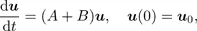
Table of contents

• Cover
• Title Page
• Copyright
• Introduction
• Chapter 1: Introduction to Arbitrary Lagrangian–Eulerian in Finite Element Methods
• Chapter 2: Fluid–Structure Interaction: Application to Dynamic Problems
• Chapter 3: Implicit Partitioned Coupling in Fluid–Structure Interaction
• Chapter 4: Avoiding Instabilities Caused by Added Mass Effects in Fluid–Structure Interaction Problems
• Chapter 5: Multidomain Finite Element Computations: Application to Multiphasic Problems
• List of Authors
• Index