Lie Groups for Pedestrians

Harry J. Lipkin

• Publisher: Dover Publications
• Year: 2012
• ISBN:
  9780486137889
• Topic: Physical Sciences
• Subtopic: Physics
• Index: Physics

According to the author of this concise, high-level study, physicists often shy away from group theory, perhaps because they are unsure which parts of the subject belong to the physicist and which belong to the mathematician. However, it is possible for physicists to understand and use many techniques which have a group theoretical basis without necessarily understanding all of group theory. This book is designed to familiarize physicists with those techniques. Specifically, the author aims to show how the well-known methods of angular momentum algebra can be extended to treat other Lie groups, with examples illustrating the application of the method.
Chapters cover such topics as a simple example of isospin; the group SU3 and its application to elementary particles; the three-dimensional harmonic oscillator; algebras of operators which change the number of particles; permutations; bookkeeping and Young diagrams; and the groups SU4, SU6, and SU12, an introduction to groups of higher rank. Four appendices provide additional valuable data.

CHAPTER 1

INTRODUCTION

Physicists have not yet learned to live with group theory in the same way as they have learned for other mathematical techniques such as differential equations. When an experimentalist or advanced graduate student encounters a simple differential equation in the course of his work, he does not run away and hide, worry about whether the solution to the equation really exists, or indulge in mathematical exercises of a ‘high-brow’ nature. He either solves the equation or goes to the literature and looks up the solution. On the other hand, many sophisticated theorists who are quite at home in the complex plane seem to be afraid of what might be called elementary exercises in group theory. This is all the more mysterious since many of these so-called group theoretical methods are in principle no different and no more complicated than certain mathematical techniques which every physicist learns in a course in elementary quantum mechanics; namely, the algebra of angular momentum operators.

The reason for this difficulty may be that physicists have still not made the separation analogous to that made for differential equations between those parts of the subject which belong to the physicist and those which belong to the mathematician. The standard treatment of group theory for physicists begins with complicated definitions, lemmas, and existence proofs which are certainly necessary for a proper understanding of group theory. However, it is possible for physicists to understand and to use many techniques which have a group theoretical basis without necessarily understanding all of group theory, in the same way as he now uses angular momentum algebra without delving deeply into the mysteries of the three-dimensional rotation group.

The purpose of this treatment is to show how techniques analogous to angular momentum algebra can be extended and applied to other group theoretical problems without requiring a detailed understanding of group theory.

1.1. REVIEW OF ANGULAR MOMENTUM ALGEBRA

Consider three angular momentum operators J_x, J_y and J_z which satisfy the well-known commutation rules

(1.1)

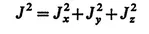
From these commutation rules it follows that there exists an operator

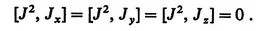
which has the property of commuting with all the angular momentum operators:

(1.2)

Since J² commutes with all the operators, it commutes with any one of them, and one usually chooses the operator J_z. One can then in any problem find a complete set of states which are simultaneous eigenfunctions of J² and J_z with eigenvalues usually designated by J and M. We use the conventional designation for these states

(1.3)

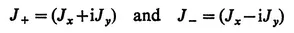
The remaining two operators J_x and J_y do not commute with J_z, but the following simple linear combinations

(1.4)

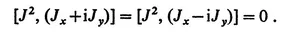
satisfy particularly simple commutation rules. Since J² commutes with all the operators, we have

(1.5)

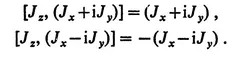
The commutators with J_z are also quite simple,

(1.6)

The commutator of each of these operators with J_z is just the same operator again, multiplied by a constant. It then follows that if either of these operators operates on a state which is a simultaneous eigenfunction of J² and J_z with eigenvalues J and M, the result is another state which is an eigenfunction of J² with the same eigenvalue J and which is also an eigenfunction of J_z, but with the eigenvalue M±1.

(1.7)

The value of the coefficient appearing on the right-hand side is easily obtained by a little algebra. This result and the trivial

(1.8)

define matrix elements for all of the angular momentum operators for all of the complete set of states.

Beginning with any particular state, |J, M〉, a set of states can be generated by operating successively with the operators (J_x+iJ_y) and (J_x–iJ_y). This process cannot be continued indefinitely because M can never be greater than J. Thus one finds restrictions on the possible eigenvalues of J and M, and obtains the well-known result that these may be either integral or half-integral and that for any eigenvalue J there corresponds a set or multiplet of 2J + 1 states all having the same eigenvalue of J and having values of M equal to–J,–J+1, ..., +J. The full set of states in a multiplet can be generated from any one of the states by successive operation with the operators (J_x±iJ_y).

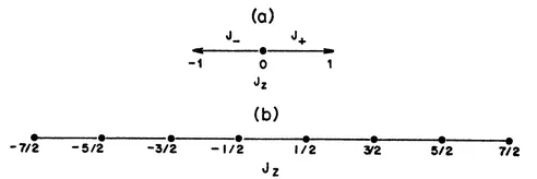
Some of these features can be demonstrated simply in diagrams of the type shown in Fig. 1.1. These diagrams are one-dimensional plots of the eigenvalues of J_z. Fig. 1.1a represents the operators (J_x+iJ_y) and (J_x–iJ_y) as vectors which change the eigenvalue of J_z by ± 1, respectively. Figure 1.1b illustrates the structure of a typical multiplet, in this case one with J =

, in which a point is plotted for each value of J_z where a state exists in the multiplet. The operation of any of the operators in Fig. 1.1a on the states in the multiplet of Fig. 1.1 b is represented graphically by taking the appropriate vector of Fig. 1.1a , placing it on Fig. 1.1b and noting which states are connected by this vector.

Fig. 1.1

There are also well-known rules for combining multiplets. A system may consist of several parts, each of which is characterized by a multiplet having a particular value of J. (An example of this would be the orbital and spin angular momenta of a particle.) These multiplets can be combined to form a multiplet describing the whole system. (For example, an orbital angular momentum of 2 and a spin of

for a particle can be combined to give a total angular momentum either of

or

.) Given the J-values for the multiplets describing parts of the system, there are simple rules for deciding which possible values of J occur for the total system, and there are algebraic techniques involving vector coupling coefficients for expressing the wave functions of the combined system which belong to a given multiplet. There is also one very simple rule which results from the different character of the multiplets having half-integral and integral values of J. If two multiplets ...

Table of contents

• Title Page
• Copyright Page
• PREFACE TO FIRST EDITION
• PREFACE TO SECOND EDITION
• Table of Contents
• CHAPTER 1 - INTRODUCTION
• CHAPTER 2 - ISOSPIN. A SIMPLE EXAMPLE
• CHAPTER 3 - THE GROUP SU3 AND ITS APPLICATION TO ELEMENTARY PARTICLES
• CHAPTER 4 - THE THREE-DIMENSIONAL HARMONIC OSCILLATOR
• CHAPTER 5 - ALGEBRAS OF OPERATORS WHICH CHANGE THE NUMBER OF PARTICLES
• CHAPTER 6 - PERMUTATIONS, BOOKKEEPING AND YOUNG DIAGRAMS
• CHAPTER 7 - THE GROUPS SU4, SU6 AND SU12, AN INTRODUCTION TO GROUPS OF HIGHER RANK
• APPENDIX A - CONSTRUCTION OF THE SU3 MULTIPLETS BY COMBINING SAKATON TRIPLETS
• APPENDIX B - CALCULATIONS OF SU3 USING AN SU2 SUBGROUP: U-SPIN
• APPENDIX C - EXPERIMENTAL PREDICTIONS FROM THE OCTET MODEL OF UNITARY SYMMETRY
• APPENDIX D - PHASES, A PERENNIAL HEADACHE
• BIBLIOGRAPHY
• SUBJECT INDEX