Electronic Structure and the Properties of Solids

The Physics of the Chemical Bond

Walter A. Harrison

• Publisher: Dover Publications
• Year: 2012
• ISBN:
  9780486141787
• Topic: Physical Sciences
• Subtopic: Physics
• Index: Physics

`Should be widely read by practicing physicists, chemists and materials scientists.` — Philosophical Magazine
In this comprehensive and innovative text, Professor Harrison (Stanford University) offers a basic understanding of the electronic structure of covalent and ionic solids, simple metals, transition metals, and their compounds. The book illuminates the relationships of the electronic structures of these materials and shows how to calculate dielectric, conducting, and bonding properties for each. Also described are various methods of approximating electronic structure, providing insight and even quantitative results from the comparisons. Dr. Harrison has also included an especially helpful `Solid State Table of the Elements` that provides all the parameters needed to estimate almost any property of any solid, with a hand-held calculator, using the techniques developed in the book.
Designed for graduate or advanced undergraduate students who have completed an undergraduate course in quantum mechanics or atomic and modern physics, the text treats the relation between structure and properties comprehensively for all solids rather than for small classes of solids. This makes it an indispensable reference for all who make use of approximative methods for electronic-structure engineering, semiconductor development and materials science.
The problems at the ends of the chapters are an important aspect of the book. They clearly show that the calculations for systems and properties of genuine and current interest are actually quite elementary. Prefaces. Problems. Tables. Appendixes. Solid State Table of the Elements. Bibliography. Author and Subject Indexes.
`Will doubtless exert a lasting influence on the solid-state physics literature.` — Physics Today

PART I

ELECTRON STATES

IN THIS PART of the book, we shall attempt to describe solids in the simplest meaningful framework. Chapter 1 contains a simple, brief statement of the quantum-mechanical framework needed for all subsequent discussions. Prior knowledge of quantum mechanics is desirable. However, for review, the premises upon which we will proceed are outlined here. This is followed by a brief description of electronic structure and bonding in atoms and small molecules, which includes only those aspects that will be directly relevant to discussions of solids. Chapter 2 treats the electronic structure of solids by extending the framework established in Chapter 1. At the end of Chapter 2, values for the interatomic matrix elements and term values are introduced. These appear also in a Solid State Table of the Elements at the back of the book. These will be used extensively to calculate properties of covalent and ionic solids.

The summaries at the beginnings of all chapters are intended to give readers a concise overview of the topics dealt with in each chapter. The summaries will also enable readers to select between familiar and unfamiliar material.

CHAPTER 1

The Quantum-Mechanical Basis

SUMMARY

This chapter introduces the quantum mechanics required for the analyses in this text. The state of an electron is represented by a wave function

. Each observable is represented by an operator O. Quantum theory asserts that the average of many measurements of an observable on electrons in a certain state is given in terms of these by ∫ Ψ*OΨd³r. The quantization of energy follows, as does the determination of states from a Hamiltonian matrix and the perturbative solution. The Pauli principle and the time-dependence of the state are given as separate assertions.

In the one-electron approximation, electron orbitals in atoms may be classified according to angular momentum. Orbitals with zero, one, two, and three units of angular momentum are called s, p, d, and ƒ orbitals, respectively. Electrons in the last unfilled shell of s and p electron orbitals are called valence electrons. The principal periods of the periodic table contain atoms with differing numbers of valence electrons in the same shell, and the properties of the atom depend mainly upon its valence, equal to the number of valence electrons. Transition elements, having different numbers of d orbitals or f orbitals filled, are found between the principal periods.

When atoms are brought together to form molecules, the atomic states become combined (that is, mathematically, they are represented by linear combinations of atomic orbitals, or LCAO’s) and their energies are shifted. The combinations of valence atomic orbitals with lowered energy are called bond orbitals, and their occupation by electrons bonds the molecules together. Bond orbitals are symmetric or nonpolar when identical atoms bond but become asymmetric or polar if the atoms are different. Simple calculations of the energy levels are made for a series of nonpolar diatomic molecules.

1-A Quantum Mechanics

For the purpose of our discussion, let us assume that only electrons have important quantum-mechanical behavior. Five assertions about quantum mechanics will enable us to discuss properties of electrons. Along with these assertions, we shall make one or two clarifying remarks and state a few consequences.

Our first assertion is that

(a) Each electron is represented by a wave function, designated as ψ(r). A wave function can have both real and imaginary parts. A parallel statement for light would be that each photon can be represented by an electric field

(r, t). To say that an electron is represented by a wave function means that specification of the wave function gives all the information that can exist for that electron except information about the electron spin, which will be explained later, before assertion (d). In a mathematical sense, representation of each electron in terms of its own wave function is called a one-electron approximation.

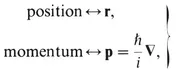
(b) Physical observables are represented by linear operators on the wave function. The operators corresponding to the two fundamental observables, position and momentum, are

(1-1)

where

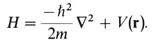
is Planck’s constant. An analogous representation in the physics of light is of the observable, frequency of light; the operator representing the observable is proportional to the derivative (operating on the electric field) with respect to time, ∂/∂t. The operator r in Eq. (1-1) means simply multiplication (of the wave function) by position r. Operators for other observables can be obtained from Eq. (1-1) by substituting these operators in the classical expressions for other observables. For example, potential energy is represented by a multiplication by V(r). Kinetic energy is represented by (

²/2m)∇². A particularly important observable is electron energy, which can be represented by a Hamiltonian operator:

(1-2)

The way we use a wave function of an electron and the operator representing an observable is stated in a third assertion:

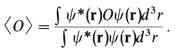
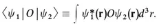
(c) The average value of measurements of an observable O, for an electron with wave function ψ, is

(1-3)

(If ψ depends on time, then so also will 〈O〉.) Even though the wave function describes an electron fully, different values can be obtained from a particular measurement of some observable. The average value of many measurements of the observable O for the same ψ is written in Eq. (1-3) as 〈O〉. The integral in the numerator on the right side of the equation is a special case of a matrix element; in general the wave function appearing to the left of the operator may be different from the wave function to the right of it. In such a case, the Dirac notation for the matrix element is

(1-4)

In a similar way the denominator on the right side of Eq. (1-3) can be shortened to <ψ|ψ>. The angular brackets are also used separately. The bra <1| or <ψ₁| means ψ₁(r)*; the ket |2> or |ψ₂> means ψ₂(r). (These terms come from splitting the word “ bracket.”) When they...

Table of contents

• Title Page
• Copyright Page
• Dedication
• Preface to the Dover Edition - Recent Developments
• Preface to the First Edition
• Table of Contents
• PART I - ELECTRON STATES
• PART II - COVALENT SOLIDS
• PART III - CLOSED-SHELL SYSTEMS
• PART IV - OPEN-SHELL SYSTEMS
• APPENDIX A - The One-Electron Approximation
• APPENDIX B - Nonorthogonality of Basis States
• APPENDIX C - The Overlap Interaction
• APPENDIX D - Quantum-Mechanical Formulation of Pseudopotentials
• APPENDIX E - Orbital Corrections
• Solid State Table of the Elements
• Bibliography and Author Index
• Subject Index