Finite Element Analysis

M Moatamedi, Hassan Khawaja

• Publisher: CRC Press
• Year: 2018
• ISBN:
  9780429841606
• Edition: 1
• Topic: Mathematics
• Subtopic: Mathematics General
• Index: Mathematics

Finite element analysis has become the most popular technique for studying engineering structures in detail. It is particularly useful whenever the complexity of the geometry or of the loading is such that alternative methods are inappropriate. The finite element method is based on the premise that a complex structure can be broken down into finitely many smaller pieces (elements), the behaviour of each of which is known or can be postulated. These elements might then be assembled in some sense to model the behaviour of the structure. Intuitively this premise seems reasonable, but there are many important questions that need to be answered. In order to answer them it is necessary to apply a degree of mathematical rigour to the development of finite element techniques. The approach that will be taken in this book is to develop the fundamental ideas and methodologies based on an intuitive engineering approach, and then to support them with appropriate mathematical proofs where necessary. It will rapidly become clear that the finite element method is an extremely powerful tool for the analysis of structures (and for other field problems), but that the volume of calculations required to solve all but the most trivial of them is such that the assistance of a computer is necessary.

As stated above, many questions arise concerning finite element analysis. Some of these questions are associated with the fundamental mathematical formulations, some with numerical solution techniques, and others with the practical application of the method. In order to answer these questions, the engineer/analyst needs to understand both the nature and limitations of the finite element approximation and the fundamental behaviour of the structure. Misapplication of finite element analysis programs is most likely to arise when the analyst is ignorant of engineering phenomena.

Chapter 1

Introduction

Chapter one introduces the aims and objectives of the book, history and perspective relating to the engineering problem, the fundamentals, numerical methods and application of the finite element method. This chapter also discusses the terminology associated with the finite element mesh.

Finite element analysis has become the most popular technique for studying engineering structures in detail. It is particularly useful whenever the complexity of the geometry or of the loading is such that alternative methods are inappropriate. This book provides an introduction to the finite element method.

1.1    Book Aims and Objectives

•  To introduce finite element analysis as a tool for the solution of practical engineering problems.

•  To teach the principles of finite element analysis, including the mathematical fundamentals as required.

•  To demonstrate how to construct an appropriate finite element model of a physical system, and how to interpret the results of the analysis.

1.2    History and Perspective

1.2.1    The engineering problem

There are three steps in the analytical solution of a physical problem:

  i)  Identify the variables.

 ii)  Formulate governing equations describing the physical system, including any constraints and boundary conditions.

iii)  Solve the equations.

A most prudent fourth step is to validate the solutions with the experimental data.

Having identified the important variables, the governing equations for the system are formulated. Depending on the physical system under investigation, these might be based on principles of conservation of mass, conservation of momentum, conservation of energy, minimum potential energy, etc. At this stage it is almost always necessary to make simplifying assumptions in order to reduce the general equations to a form for which solutions can be sought.

Historically, many eminent mathematicians and scientists have formulated and solved governing equations for specific physical systems. It has often been necessary to invoke knowledge of empirical relationships between variables in order to generate acceptable solutions. Every engineering textbook is full of equations bearing the names of individuals who first developed the associated theories, and it is possible to gain a strong insight into the performance of most physical systems by performing calculations using these equations. Closed form solutions are available for many practical engineering problems, and until the late 1950s all engineering design analysis was based on such solutions. The introduction of the digital computer to engineering applications started a revolution in design analysis that is still gathering momentum. The ability of the computer to solve large systems of simultaneous equations led to the development of matrix methods for structural analysis problems, and these in turn led to the development of finite element analysis methods.

1.2.2    The finite element method

The finite element method is based on the premise that a complex structure can be broken down into a finite number of smaller pieces (elements), the behaviour of each of which is known or can be postulated. These elements might then be assembled, in some sense, to model the behaviour of the structure. Intuitively, this premise seems reasonable, but there are many important questions that need to be answered. In order to answer them, it is necessary to apply a degree of mathematical rigour to the development of finite element techniques. The approach that will be taken in this book is to develop the fundamental ideas and methodologies based on an intuitive engineering approach, and then to support them with appropriate mathematical proofs where necessary. It will rapidly become clear that the finite element method is an extremely powerful tool for the analysis of structures (and for other field problems), but that the volume of calculations required to solve all but the most trivial of them is such that the assistance of a computer is necessary.

It has been mentioned above that many questions arise concerning finite element analysis. Some of these questions are associated with the fundamental mathematical formulations, some with numerical solution techniques, and others with the practical application of the method. A short list of questions is presented below to give an indication of the issues that are important to the developers and users of this powerful analysis technique.

Fundamentals:

•  Are there any restrictions on the postulated behaviour of the individual elements?

•  Is convergence guaranteed? (i.e., does the accuracy of the solution improve as the structure is divided into more and more elements?)

•  Can the intrinsic error in a finite element solution be estimated, or at least can it be bounded? Under what circumstances might the error be zero?

Numerical methods:

•  The finite element method will require the solution of a potentially very large set of simultaneous equations. What algorithms are most appropriate for their solution, and how can the resources required be minimised?

•  What restrictions on accuracy are imposed by numerical solutions—can they be estimated or bounded?

Application:

•  How accurately does the model geometry need to reflect the actual geometry? Is it necessary to model local geometrical features such as fillet radii?

•  How many elements, and of what type, are needed to analyse a particular structure under a particular set of loads?

•  How might the resources required for an analysis be estimated?

In order to answer these questions, the engineer/analyst needs to understand both the nature and limitations of the finite element approximation and the fundamental behaviour of the structure. Misapplication of finite element analysis programs is most likely to arise when the analyst is ignorant of engineering phenomena.

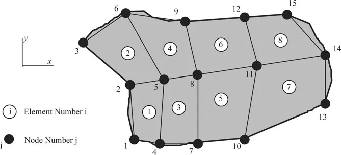
1.3    The Finite Element Mesh: Terminology

Figure 1.1 Description of Finite Element Mesh.

The physical domain (bounded by the bold line in Fig. 1.1) is broken down into discrete elements. At the boundaries of the domain, there is some approximation of the geometry unless the shape of the element edges corresponds exactly to the shape of the boundary.

The shapes of the elements are determined by the positions and connectivity of nodes. For simple triangular elements the minimum number of nodes required to define their shape and position is three (one at each corner). The simple quadrilaterals illustrated above are defined by the positions of the four corner nodes. More complex elements can be defined using more nodes: for example, an eight node quadrilateral can have curved edges defined by positions of mid-side nodes.

When the structure is loaded, each node can move from its original location. If the node is considered as a small solid particle there are six possible displacements in three dimensions. It can translate in any direction, and in general this translation will have a component along each of the three global axes. It can also rotate, and similarly the rotation has a component about each of the three global axes. Each of the components of translation and rotation is referred to as a degree of freedom, and in three dimensions each node, therefore, has six degrees of freedom. The number of active degrees of freedom at each node depends on the formulation of the elements connecting the nodes. If the area illustrated above represents a membrane in the xy plane, each node will have two active degrees of freedom: they are translation in the x direction (u), and translation in the y direction (v). The finite element model illustrated would, therefore, have 15 × 2 = 30 degrees of freedom.

Chapter 2

Matrix Stiffness Methods

The displacement-based finite element method is closely related to the matrix stiffness methods that were developed in the late 1950’s in order to exploit the newly-arrived digital computers. Many of the procedures that are important in finite element analysis can be illustrated cl...

Table of contents

• Cover
• Title Page
• Copyright Page
• Table of Contents
• Preface
• 1. Introduction
• 2. Matrix Stiffness Methods
• 3. The Finite Element Formulation: One-Dimensional Problems
• 4. The Finite Element Formulation: Two-Dimensional Problems
• 5. Computational Implementation of the Finite Element Method
• 6. Beams, Plates, Shells and Solids
• 7. Parametric Element Formulations
• Suggested Reading
• Index