Moneynomics

The Evolution of Money in Theory, Practice, and Policy

Steven Ricchiuto

• Publisher: Greenleaf Book Group Press
• Year: 2020
• ISBN:
  9781626347175
• Topic: Economics
• Subtopic: Economic History
• Index: Economics

A Comprehensive Look at the Evolving Role of Money in Our Economy Steven Ricchiuto, Wall Street veteran and US economist, shares with you his expert knowledge about the diverse history and function of money in the US economy. Tracing the development of money from shells to today’s fiat currency regime, Ricchiuto dissects the different models economists use to explain money’s role in the economy and how it determines growth, inflation, and interest rates.  Moneynomics is the only book you need for understanding money’s changing purpose in the economy. Inside is a detailed explanation of all aspects of money, including:

• The various forms money has taken throughout history

• Why gold has long been a favored form of money

• The role money plays in the economy—theoretically, in practice, and in policy

• How you can use the lessons learned in the past to understand how we have gone from battling stagflation to trying to stave off deflation

• Recognizing the shifting functions of money in the evolution of macroeconomic theory and the different forms of currency regimes  ?Using Ricchiuto’s vast experience and acumen, you, too, can become an authority on the role of money in our world, and how it ultimately impacts your life and the overall economy.

Section 1

The Theoretical Role of Money in the Economy

Chapter 1

The Keynesian IS–LM Model

Money plays a central role in macroeconomic theory. In this chapter, we examine the first highly influential model of the economy where money was a key policy lever that could be manipulated to move an economy from one short-term equilibrium to another.

The genesis of this model can be traced to the work done by John Maynard Keynes during the late stages of the Great Depression (1929–1939) and presented in his General Theory of Employment, Interest Rates and Money published in 1936. According to Keynes’s work, the Depression was caused by a widespread loss of confidence that led to underconsumption. Once panic and deflation set in, many people believed they could avoid further losses by steering clear of markets. Holding money became profitable as the price of goods and services dropped, suggesting that holding cash could allow individuals to buy more later. This dynamic became known as the Keynesian Liquidity Trap.

The macro dynamic outlined by Keynes in his General Theory was further developed by John Hicks in 1937 and later extended by Alvin Hansen into the mathematical model that would become the framework behind the macroeconomic theory between the 1940s and the 1970s, and is still the backbone of most introductory macroeconomics textbooks. The IS–LM model, or Hicks-Hansen model, shows the relationship between interest rates and real income that brings both markets for goods and services into alignment with those that are consistent with equilibrium in the liquidity market. The equilibrium in the liquidity market is dependent on the level of money provided to the economy by the Federal Reserve. As such, the IS–LM model shows that monetary policy could be exploited just as easily as fiscal policy for countercyclical purposes.

Basic Model Framework

The model is presented graphically as the intersection of two curves. One curve identifies the pairs of income and interest rates that identify possible equilibrium conditions in the market for goods and services, and the other identifies the conditions for equilibrium in the liquidity market. The level of income and interest rates that satisfies both markets simultaneously is the estimated short-term equilibrium for the economy. The IS (investment-saving) curve identifies pairs of income and interest rates that will result in equilibrium in the goods and services market. The equilibrium position is defined as the point where savings equals investment in the economy. When working through the various pairs of income and interest rates that satisfy the demand for consumer and investment goods under an equilibrium condition, the savings rate needs to equal investment so a downward-sloping IS curve is traced out.

The LM, or liquidity curve, determines the income and interest-rate pairs that satisfy the condition that demand for money equals the supply of money in the economy. The intersection between the downward-sloping IS curve and the upward-sloping LM curve is seen as the short-term equilibrium of the economy. Movement from one equilibrium to another can be generated by a policy-induced shift in either the IS or the LM curve. This will result in a different equilibrium pair of income and interest rates for the economy. Because we are considering short-term equilibrium, inflation is seen as having a limited effect on the economy, and the equilibrium pairs of income and interest rates are identified as real, or inflation adjusted, rather than nominal. To better understand this model, a brief but thorough discussion of the determinants of the IS and LM curve will prove useful and allow us to better understand the central role money plays in how the economy works, without getting overly technical.

Equilibrium in the Goods Market

The IS curve is a simple statistical model that depicts the level of real interest rates and real GDP or aggregate income that generate equilibrium in the markets for goods and services. These interest-rate and aggregate income pairs satisfy the following equation, subject to the equilibrium condition that savings equals investment:

Here, Y represents real GDP and C(Y − T(y)) represents consumer spending as an increasing function of disposable income (Y − T(Y)); that is, the partial derivative of consumption with respect to disposable income is greater than zero. I(R, Y) represents investment spending as a decreasing function of the real interest rate and an increasing function of real income; in other words, the partial derivatives of investment spending are negative for changes in real interest rates and positive for changes in real income. G represents government spending, which is set exogenously by the interaction of Congress and the administration. We could add a real asset variable as a positive determinant of consumer spending as well as net exports to the model, but for our purposes, these modifications are unnecessary. However, the difference between exports and imports would be a decreasing function of real income, or Y, since (1) the level of imports is positively related to real income; and (2) exports depend on factors outside this model.

The above equation can be rewritten as

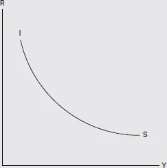
S represents total savings and is a positive function of real income. In product market equilibrium, total savings (private plus government) must be equal to total investment including that undertaken by the government. The real income and interest-rate pairs that satisfy this equilibrium condition form the IS curve, or half of the Hicks-Hansen model of the macro economy. It should be noted that upward shifts in the IS curve can be generated by an increase in the relative desire to invest in new plant and equipment at any given level of interest rates, or by an increase in government spending. A reduction in the desire to consume for every dollar earned, or an increase in the desire to save, also shifts the IS curve upward and to the right; while a reduced sensitivity of investment to interest rates flattens the IS curve. The IS curve is not a complete model of equilibrium in the economy, in that it doesn’t ensure equilibrium in liquidity markets, and therefore, in the labor market either. These will be discussed below.

fig 1.1

IS Curve

Equilibrium in the Liquidity Markets

The LM curve shows the pairs of income and interest rates for which the money or liquidity market is in equilibrium, that is, where the demand and supply of money in the economy are in balance. This equilibrium curve is seen as upward sloping, representing the role of money and finance in the economy. Equilibrium in the liquidity market is determined by solving the following equation:

MS(R) represents the supply of money provided to the economy by the Federal Reserve through the banking system. As rates rise, the banking industry tends to be more willing to provide additional loans to would-be borrowers and the supply of money to the economy increases through the level of demand deposits generated by banks. The aggregate price level in the economy is denoted by the letter P. It is essentially the price index that deflates nominal GDP to real GDP. Money demand, MD(Y, R), can be interpreted as the sum of the speculative demand for money (which is negatively dependent on the level of interest rates) and the transactions demand of money (which is positively dependent on the level of income). As income in the economy tends to increase, the interest rates needed to keep the liquidity market in equilibrium tend to increase as well, giving the LM curve its positive slope.

The elasticity the LM curve exhibits depends on the sensitivity of the speculative demand for money to changes in interest rates. The flatter the speculative demand for money, the flatter the LM, and vice versa. Alternatively, the less sensitive the supply of money is to the level of interest rates, the more the LM curve shifts up and to the left. This equilibrium relationship shows the important role money plays in the economy, as it is key to the interaction between the product and money markets and can be manipulated to alter the level of aggregate demand in the economy. This will be seen more clearly in the following section.

fig 1.2

LM Curve

Product and Liquidity, Money Market Equilibrium

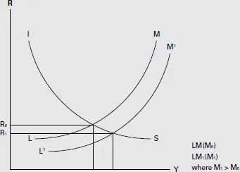
By simultaneously solving the IS and the LM equations for the level of output and interest rates that clear both markets, we get the level of real GDP that is associated with a given price level, or a single point on the aggregate demand curve. Also, note that G, government spending, and P, the aggregate price level, are two of the three exogenous variables in this model. Increasing G results in a higher level of output at a given level of prices. Increasing real money balances in the economy can accomplish a similar outcome of higher real GDP.

fig 1.3

IS–LM

Increasing or decreasing the aggregate price level, and calculating the equilibrium level of GDP consistent with equilibrium for the product and the liquidity markets, traces out an aggregate demand curve. By combining this aggregate demand relationship with an aggregate supply determined by the labor market condition (i.e., a Phillips curve), a complete model of the economy was constructed. This model became the basis behind all macroeconomic thinking in the postwar period, until it fell out of favor due to the era of stagflation that surfaced in the late 1970s and early 1980s. The labor market model was not capable of anticipating the changed dynamic between employment and inflation expectations that developed thirty years into the postwar period. This development required a new interpretation of how the economy functions. These new theories had to explain how prices could rise in an environment in which slack in the labor market was increasing (a rising jobless rate). This will be discussed in more detail in Chapter 3, Stagflation and the Rise of Monetarism.

Ascendance of Fiscal and Monetary Policy

The intuitive nature of the IS–LM aggregate demand/aggregate supply framework explains why policy makers relied heavily on this model from the 1940s through 1970s and even today, to some extent. For instance, the Trump/GOP Tax Cuts and Jobs Act of 2017 is a modern-day example of trying to exploit the macro framework depicted by the Keynesian model to increase employment and lift the economy to a higher growth trajectory. The ease with which the various components of the model can be manipulated to simulate various macroeconomic and policy scenarios led to the belief among economists in the 1950s and 1960s that the business cycle could be dampened or even eliminated entirely with the right sequence of fiscal and monetary policy stimuli. The evolution of computers extended the life of the IS–LM framework, even when signs of the model’s limitations began to surface. The Keynesian model identified by Hicks and Hansen could be easily modified to correct for certain errors, and the speed of computers in manipulating large data sets broadened the scope of the model to simulate results of policy changes not just at the sector level, but also at the industry and sub-industry level.

The Keynesian model, moreover, was the justification behind Roosevelt’s New Deal programs enacted during the Depression. Programs like the Works Progress Administration (WPA) were the first concerted fiscal stimulus programs enacted. Unfortunately, it appears these early attempts at countercyclical policies were too small in scope to offset the monetary contraction that followed in the wake of some 9,000 Depression-era bank failures. The fact that Fed policy did not support the Roosevelt stimulus initiative is seen as a missed opportunity, and it shaped the postwar focus of monetary policy that emphasized controlling the level of interest rates in the economy as the means to maximizing growth and sustaining full employment. Essentially, monetary policy best serves the economy if it supports the fiscal policy decisions by elected officials by maintaining low short-term interest rates.

In the period following the conclusion of World War II, fiscal policy was used repeatedly to alter the trajectory of the economy. The so-called Kennedy tax cut enacted by President Johnson in 1964 is a well-publicized example of a Keynesian-inspired tax cut. At that time, the Fed saw its responsibility as supportin...

Table of contents

• Cover
• Title
• Copyright
• Contents
• Preface
• Acknowledgments
• Introduction
• Section 1 The Theoretical Role of Money in the Economy
• Section 2 The Practical Side to Money in the Economy
• Section 3 Money’s Role Reversal
• Conclusion What’s Next?
• About The Author