First (and Second) Steps in Statistics

Daniel B Wright, Kamala London

• Publisher: SAGE Publications Ltd
• Year: 2009
• ISBN:
  9781446242780
• Edition: 2
• Topic: Ciencias sociales
• Subtopic: Investigación y metodología de las ciencias sociales

?This engagingly written and nicely opinionated book is a blend of friendly introduction and concisely applicable detail. No-one can recall every statistical formula, but if they have this book they will know where to look? - Professor Jon May, University of Plymouth

?This is one of the best books I have come across for teaching introductory statistics. The illustrative examples are engaging and often humorous and the explanations of ?difficult? concepts are written in a wonderfully clear and intuitive way? - Nick Allum, University of Essex

Selected as an Outstanding Academic Title by Choice Magazine, January 2010

First (and Second) Steps in Statistics, Second Edition provides a clear and concise introduction to the main statistical procedures used in the social and behavioural sciences and is perfect for the statistics student starting their journey.

The rationale and procedure for analyzing data are presented through exciting examples with an emphasis on understanding rather than computation. It is ideally suited for introductory courses in statistics given its gentle beginning, yet progressive treatment of topics. In addition to descriptive statistics, graphs, t-tests, oneway ANOVAs, Chi-square, and simple linear regression, this Second Edition now includes some new, more advanced topic areas as well as a host of additional examples to help students confidently progress through their studies and apply the techniques in lab work, reports and research projects.

Key features of this new edition:

- the reoganization of the first three chapters giving more attention to univariate statistics and providing more examples to work through at this level

- more advanced ?second step? content has been added on factorial ANOVA and multiple regression

- the robust methods chapter from the first edition is now spread throughout the book, and is linked with common teaching practices.

- many more examples have been added to enhance the book?s practical potential.

- a host of exercises as well as further reading sections at the end of every chapter.

An accompanying Web page includes information for each chapter using the statistical packages SPSS and R.

1

Univariate Statistics 1: Summarizing Data with Histograms and Boxplots

Example: DNA Exonerations

Histograms

The Five-Number Summary

Summary of the Five-Number Summary and Boxplots

Conclusions

Exercises

Further Reading

The art of statistics is both about discerning patterns in data and about communicating information about these patterns to an audience. Statistics is an art, but that does not mean that anything goes. Like other artists you need to learn technical skills and guidelines in order for your art to be any good. To take an extreme example: go to GOOGLE and IMAGE and put in ‘Jackson Pollock’. Jackson Pollock was considered one of America’s best twentieth-century artists and was most well known for a brand of abstract expressionism where he appeared to drip paint in a chaotic and undisciplined manner over a canvas. However, his technical abilities are clearly shown in his earlier paintings, and it was only with these skills that he could venture into an unexplored artistic genre. This book will not turn you into the Jackson Pollock of statistics, but it will help you to learn the basic tools of the trade and how to apply them. While painters, sculptors and poets have certain tools at their disposal, as a statistical artist you have various tools to facilitate both the discovery and the dissemination of your findings. Statistics is not just about what you can do with data; it is also about how you describe what you found to your expected audience. Therefore, your toolbox must include knowledge about your audience, as well as the more traditional tools like a pen and paper, and some computer software.¹

This book introduces a language that allows us to talk about statistics, and science more generally. This is not a completely foreign language. Statistical phrases permeate our daily lives. Usually these are not the ‘formal’ statistics that appear in statistics books and in scientific reports, but they are embedded, very innocently, in our conversations. Examples include phrases like ‘I will probably have a bagel today’ and ‘It takes about 20 minutes to cook rice’. The aims of this book are to enhance your awareness of these natural language statistics, to allow you to translate these into ‘formal’ statistics and, in so doing, to enable you to conduct, interpret and describe these statistics.

Consider the two examples mentioned above. Regardless of how likely you think it is that you will have a bagel today, you know roughly what the above statement means. When we use words like ‘probably’ we are not usually worried about the precise meaning of the phrase. Translating from natural language to formal statistics often involves becoming more precise. Here we might say that the probability of having a bagel is more than 0.50 or 50%. Probability is at the heart of statistics and will be described throughout this book. If you had a standard deck of 52 cards, shuffled them thoroughly and were about to draw one card, the probability of it being red is 0.50. So using this analogy, the above statement means that it is more likely that you will have a bagel than randomly choosing a red card from a well-shuffled deck of cards.

The second statement, ‘It takes about 20 minutes to cook rice’, is a statistical phrase because of the word ‘about’. Depending on the amount and type of rice, the initial heat of the water, the type of stove and even the altitude at which you are cooking, the amount of time it takes to cook rice is not constant, but varies. Translating this into statistics it becomes ‘Twenty minutes is the central tendency for the time to cook rice, but the exact time may vary from this’. ‘Central tendency’ is what the statisticians would call the instructions written on the side of the rice box suggesting how long to cook the rice. It is the value that, across all situations, the rice manufacturers think is the best guess for proper cooking time. There are different and more precise ways of calculating the central tendency including the median, which is discussed in this chapter, and the mean, which is discussed in Chapter 2.

For most of you, the main concern with regards to statistics is not to help you to become a better rice chef, but how statistics are used and reported in the social and behavioural sciences. The point of these examples is to show how frequently statistics are encountered in our lives. During the course of your studies you will come across other ‘everyday statistics’ and also more formal statistics. This book describes various procedures for creating these statistics.

EXAMPLE: DNA EXONERATIONS

Imagine you are walking home one evening. You can hear police sirens in the background, but you don’t think much of them. A police officer approaches and asks you a few questions. A woman has been raped and the police are looking for her attacker. You say you were at a friend’s house and have been walking home. The police officer takes your name and contact details, and you go home. The next day another officer arrives at your home, and tells you that you match a rough description that the victim gave of the culprit. They ask you if you will take part in an identification parade. You agree, after all, you’re not guilty; the victim won’t choose you. Perhaps you would be less calm if you knew what the US Attorney General, Janet Reno, said in the preface to a report about eyewitness accuracy: ‘Even the most honest and objective people can make mistakes in recalling and interpreting a witnessed event’ (Technical Working Group for Eyewitness Evidence, 1999: iii). The victim identifies you as her assailant, and because jurors trust eyewitness testimony (a lot more than they should), you are convicted and spend years in prison. You may not feel lucky, but in one way you are. The crime that you were falsely convicted of is one that often includes a biological marker, semen. A DNA test is done, which shows that you are not the culprit, and, after some further legal arguments, you are eventually exonerated and released.

Your case is a tragedy of injustice, but you are not alone. The Innocence Project in the US reports hundreds of people who have been falsely convicted but later exonerated based on DNA evidence (www.innocenceproject.com). We will look at the first 163 which we downloaded on 17 November 2005. Each of these individuals’ cases is a tragedy, and it is important that when you report your statistics you do not lose sight of the meaning of each case. Each individual spent years in prison, falsely accused. As voiced by Uncle Tupelo: ‘Handcuffs hurt worse when you’ve done nothing wrong’ (‘Grindstone’ by Farrar and Tweedy).

The length of time in prison of these 163 people (the data file, dnayears.sav, is on this book’s website) will be used to illustrate some of the basic statistical concepts and graphs.

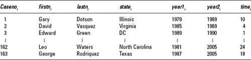
Each of the individuals in the DNA file is a case. The sample is composed of the 163 cases. The larger population in this example would be all falsely convicted individuals exonerated by DNA evidence. There is information about several attributes for each of the cases. Each of these attributes is called a variable. For this example there are seven variables: the case number, the person’s first and last name, the state where they were convicted, the year they were convicted, the year they were released, and the time between conviction and release. Each person has a value for each variable, thus for the first person, Gary Dotson, the value for state is ‘Illinois’ and for time is 10 years. Most of the values that are used in this book are numeric, but the values can also be words, pictures, etc. The way that we will refer to variables is by giving them a name that describes them, writing them in italics, and including a subscript which tells us that people may have different values for this attribute. So, the variables state_i and time_i refer to the variables denoting the state in which the person was convicted and the time they spent in prison. The subscript i shows that there are different values for these variables, the i referring to different people in the sample. If you are referring to the first person the subscript 1 is used. Thus, state₁ = ‘Illinois’ and time₁=10 years. For numeric values it is important to include the units of measurement so that it is clear that Gary Dotson spent 10 years in prison, rather than, say, 10 months in prison.

Table 1.1 The DNA cases from the Innocence Project e_i

The values for all the people in the sample, when placed together, form a data set. Most of the common statistical packages hold the data set in a spreadsheet format, like Table 1.1. Each row represents a single individual. The ‘∶’ means that the values for cases 4 to 161 are not included. It is a big data set, so would take up a lot of room to print and would be difficult to get a summary feeling for the data. This is one of the purposes of statistics, to identify useful summary information and to describe this to others.

One of the major objectives of statistics is to accurately summarize large quantities of data so that the reader can understand the overall patterns of responses. Two main types of techniques for summarizing data will be described in this chapter. The first technique is a histogram. Several variations are discussed. First a dot histogram and a stem-and-leaf diagram are shown. Then we present a generic histogram and a name histogram. The second technique is based on the five-point summary and is called a box-and-whiskers plot (or just boxplot). Both of these methods are appropriate for describing quantitative data (whe...

Table of contents

• Cover Page
• Title
• Copyright
• Contents
• Preface
• Illustrations
• Acknowledgements
• 1 Univariate Statistics 1: Histograms and Boxplots
• 2 Univariate Statistics 2: The Mean and Standard Deviation
• 3 Univariate Statistics 3: Proportions and Bar Charts
• 4 Sampling and Allocation
• 5 Inference and Confidence Intervals
• 6 Hypothesis Testing: t Tests and Alternatives
• 7 Comparing More than Two Groups or More than Two Variables
• 8 Regression and Correlation
• 9 Factorial ANOVAs and Multiple Regression
• 10 Categorical Data Analysis
• Appendix A The r Table
• Appendix B The Normal (z) Distribution
• Appendix C Student’s t Distribution
• Appendix D The F Distribution
• Appendix E The χ2 Distribution
• Appendix F How to Produce a Bad Results Section
• References
• Index