Food Product Design

A Computer-Aided Statistical Approach

Ruguo Hu

• Publisher: Routledge
• Year: 2017
• ISBN:
  9781351447553
• Edition: 1
• Topic: Technology & Engineering
• Subtopic: Food Science
• Index: Technology & Engineering

Statistical experimental design is currently used as a quality control technique to achieve product excellence at the lowest overall cost. It can also function as a powerful tool to optimize food products and/or processes, to accelerate food development cycles, reduce research costs, facilitate the transition of products from research and development to manufacturing and troubleshoot manufacturing problems. Food Product Design: A Computer-Aided Statistical Approach familiarizes readers with the methodology of statistical experimental design, and its application in food product design, with the aid of commonly available modern commercial software.Food Product Design presents basic concepts of food product design, then focuses on the most effective statistical techniques and corresponding computer applications for trial design, modeling, and experimental data analysis. The book presents very few theories about mathematics and statistics. Instead, it contains detailed descriptions of how to use popular computer software to solve the real mathematical and statistical problems that occur in product design. Even those with very limited knowledge of statistics and mathematics will find this a useful and highly practical book. Food Product Design: A Computer-Aided Statistical Approach will be a valuable tool for professional food engineers, technologists, scientists, and industrial personnel who want to update and expand their knowledge about computer-aided statistical methods in the field of food product design. Those involved in applied research at universities in food and agriculture, biological and chemical engineering, and statistics will also find it useful and informative.

CHAPTER 1

Introduction

1.1 Problems of Food Product Design

IN the field of industrial food production and processing, the problem of optimization always arises, dealing with design, development, and quality management of food products. The attempt to develop a new food product or to improve the quality of a food product that largely meets the needs of consumers proves to be appealing and challenging. General questions about food product design could include:

(1) How can changes in one set of processing variables affect overall food quality? How are they correlated to each other? Which relationships are most important for food
quality management?

(2) Which food raw materials and recipes should be used for production of an optimum quality food product? About 60–70% of the cost of most food products can be ascribed to the cost of raw materials.

(3) Which processing conditions must be used to achieve effective and successful production of a food product? Is an existing process running under control? Energy balances, likewise, are important, not because energy is a large cost factor in food processing, although it can be significant, but because correct application of energy may be the key to optimization of a process. Such important and unique processes as sterilization, pasteurization, freezing, drying, evaporation, baking, cooking, blanching, and frying all involve the addition or removal of heat to or from foods. Precise delivery of the correct amount of energy is important because both too much and too little energy transfer can be harmful.

(4) How can we determine the cause of food product defects and further control them? About 80% of all food quality defects are in part located in the design phase. One approach to track down potential problems and wrestle them under control before start-up of production is to design product quality right into the product.

(5) Most food products contain numerous ingredients, and manufacturing the product typically involves several different processing steps. How to choose the right combination of ingredients and processing steps which are important factors affecting different quality indices and desired quality characteristics of the food product?

(6) Are the recipes and the processing conditions currently used for an existing food product the best? How can we modify them to improve the food quality and/or to better meet the demands of the market? Once an optimum product has been developed, it will not remain so for all times. Usually, the quality of existing food products must be improved or modified with time to meet ever-varying consumer requests.

(7) What measures can be taken to increase production yield? How can we reduce the production cost and time of an existing food product?

(8) Is it possible to have a successful food product with cost-effective raw materials and procedures? How can individual production process be improved and wastes be minimized to improve the overall manufacturing process?

The demand for new food products and for high food quality requires extensive use of effective statistical experimental approaches by engineers and scientists. In the past, such an extensive use had been hindered due to a lack of proper training and, due to a lack of availability of appropriate computer hardware and software to implement experimental design and data analysis. This situation has now dramatically changed. Computer-aided statistical food product design will considerably improve the overall effectiveness of food research and development and enhance its application in the food research. In fact, any technique that could potentially improve the probability of a product's success in the marketplace is extremely attractive. If a particular product has optimal quality indices, such as sensory, nutritional, textural or physical, chemical and analytical attributes, it would lead to a better consumer acceptance. The attainment of optimized indices in a food product alone, of course, does not guarantee success in the marketplace, because factors, such as price, quality, brand, advertising, competition, loyalty, and economic factors, are additional major contributors to food product marketing success.

To achieve the objective of developing food products with optimal quality, we must first identify the properties and levels that are important to a specific food quality. It is important to keep in mind that optimal food products may not be able to be achieved uniquely through a combination of different product characteristics. To find out the optimum recipe and processing conditions for food products of high quality and high marketability is the critical issue. There are different methods to attain this objective, but hardly any of them can match the efficiency and the success of research and development activity in successfully supplying new and modified existing products. Among them, the statistical experimental methods such as Response Surface Methodology (RSM) are effective methods for food product design.

The theories of statistical experimental approaches have been developed for quite some time. However, they are not widely used for two main reasons. First, people in general are afraid of "statistics" and "mathematics" and, thus, avoid these methods and do not understand them. The other primary cause is the lack of suitable computer hardware and well-designed software, but this situation is rapidly changing. One of the objectives of this book is to familiarize the reader with statistical experimental methods and use them, with the aid of modern computer software, in food product design.

1.2 Classical One-Factor Experimental Method

Food process and recipe optimization is the essential task for food product designers. To accomplish this task, conventionally the One-Factor-at-a-Time Method, or One-Factor Method, is used, in which, at the first stage, only one variable is changed and tested at several levels more or less systematically, holding the other variables constant. In this way, the effect of this variable on product quality can be investigated, and a limited "optimum level" for this tested variable can be found by comparing the response results obtained. In the second stage, the optimum of a second variable can be determined. The level of the first variable is kept at its found optimum, whereas the effect of another variable is tested over several levels, while holding the rest of the variables at their constant levels. Thus, the optimal levels for each variable are found, and together they form the overall optimum for the specific product quality. This cycle is normally repeated until no significant improvement of the food quality can be detected.

This One-Factor Method is also known as the Trial & Error Method and has been used in the field of food product development for a long time. For example, salt, sugar, and smoke flavor are the major ingredients or variables responsible for most bacon flavors. Using this method to find the optimum flavor, one would change each of these variables (salt, sugar, and smoke flavor) individually, until a bacon formulation with the best flavor is achieved. In practice, the effect of salt would be tested by changing its level in the bacon while maintaining constant sugar and smoke levels and the product with the optimum flavor is selected. The optimal salt and smoke levels are then determined in a similar way. The "optimal levels" of salt, sugar, and bacon flavor would then be combined and considered as the overall optimum.

The obvious disadvantage of this experimental optimization method is its laborious experimental manner. The experimental points in the design space are not selected in a systematically structured way, and there is a low level of information extracted for experimental data collected. There is neither information about variable interaction effects nor an overview of the variables' behavior within the entire experimental space. The achieved optimum consists only of variable levels that were actually tested. This experimental method could lead an inexperienced product developer to unreliable or even false optimal results, depending on if there are significant interaction effects between the variables, which is usually the case. In the above example, the change in sugar and/or bacon flavor levels would probably modify the optimal salt level; therefore, the "overall optimum" achieved might not be the true optimum.

TABLE 1.1. Results of Five Trials of Proofing Time with T = 25 C.

Another obvious disadvantage of the Trial & Error Method is that it is inefficient and uneconomical. Usually, a large number of trials are required, especially if there are more than three variables to be investigated at multilevels, resulting in an expensive and time-consuming process. Additionally, a mathematical model would not be established by this method, so the overall relationship between the variables and the food quality (responses) could not be described quantitatively. Because food experiments in industry usually involve a large number of variables, use of designed experiments can cut the amount of costly experimentation substantially by reducing the number of trials needed to achieve a given objective.

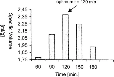
Figure 1.1 Optimum time by One-Factor Method.

To demonstrate the One-Factor-at-a-Time Method more clearly, an example is given below. The proofing time, t (mm), and the proofing temperature, T(^°C), are the two important independent variables influencing the specific volume, V (ml/g), of the loaf in the proofing process of breadmaking. The question here is: How can a proofing time and proofing temperature be found that will lead to production of a loaf with maximal specific volume? Based on pertinent literature and experience, a proofing temperature of 25–30°C was deemed reasonable. Following the approach of the One-Factor-at-a-Time Method, the proofing temperature, T, was held constant at 25°C, and the proofing time, r, varied from 60 to 180 minutes, with results that suggested that the best specific volume was obtained at 120 minutes (Table 1.1 and Figure 1.1).

TABLE 1.2. Results of Five Trials of Proofing Temperature with t = 120 min.

To investigate the effect of proofing temperature, proofing time was held constant at 120 minutes, and proofing temperature varied from 20 to 40°C. Results suggested an optimal temperature of 30°C, which gave the maximum loaf specific volume of 2.53 ml/g (Table 1.2 and Figure 1.2). Thus, the optimum proofing time and temperature appeared to be 120 minutes and 30°C. In reality this conclusion is unfortunately inexact or incorrect. The true optimum levels should be about 32°C and 90 minutes as obtained through the statistical experimental method. The statistical results are plotted by using a contour graph in Figure 1.3, in which the optimization steps and results of the One-Factor Method are illustrated. In the graph the points numbered from (1) to (10) correspond to the "Trial No." in Tables 1.1 and 1.2 in the Trial & Error optimization method.

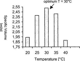
Figure 1.2 Optimum temperature by One-Factor Method.

The reason that these different results were obtained is because significant quadratic and interaction effects exist between proofing time and proofing temperature on the loaf volume. The true relationship between these variables is shown in Figure 1.4. The term interaction should be explained here. If the effect of proofing temperature on the loaf volume (response) depends on the levels of the proofing time, then there are interaction(s) between proofing time and temperature. In the One-Factor Method the interactive effect between any two independent variables is not considered, and the whole relationship is seen as described in Figure 1.5.

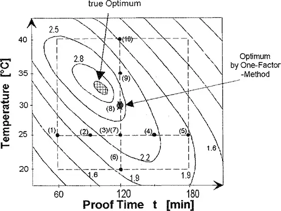
Figure 1.3 True overall relationship between the loaf specific volume and the proofing time (t) and temperature (T) (showed by contours); trial points of One-Factor Method [(1)-(10)].

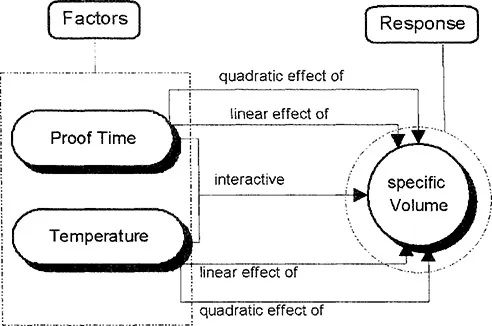
Figure 1.4 True relationship in the system.

To offset the possible disadvantages of the conventional one-factor experimental methods, efforts have been made to develop new and more effective experimental methods based on statistical disciplines for purposes such as product design, process modeling, and optimization. In these modern methods the main and the interactive effects of every independent variable are considered and checked, that is, overall relationships in the whole experimental space are determined and described in the form of mathematical models. The total number of experimental trials is reduced considerably compared with the classical Trial & Error Method, and there is no significant limiting of information value or precision with the results obtained. With the current availability and use of powerful personal computers and user-friendly statistics-oriented software, complicated calculations and graphics that proved almost impossible in the past can now be done with great ease.

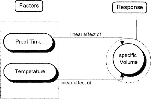
Figure 1.5 Assumed relationship in the system.

1.3 General Remarks About Statistical Methods

An alternative and modern approach of solving food product desig...

Table of contents

• Cover Page
• Title Page
• Copyright Page
• Dedication
• Contents
• Preface
• 1. INTRODUCTION
• 2. PROBLEMS OF FOOD PRODUCT DESIGN
• 3. FOOD PROCESS MODELING AND OPTIMIZATION
• 4. FOOD RECIPE MODELING AND OPTIMIZATION
• 5. MODELING AND OPTIMIZATION FOR BOTH FOOD RECIPE AND PROCESS
• 6. EXPERT SYSTEM FOR FOOD PRODUCT DEVELOPMENT
• Bibliography
• Appendix
• Index