Topographic Laser Ranging and Scanning

Principles and Processing, Second Edition

Jie Shan, Charles K. Toth, Jie Shan, Charles K. Toth

• Publisher: CRC Press
• Year: 2018
• ISBN:
  9781351650427
• Edition: 2
• Topic: Technology & Engineering
• Subtopic: Civil Engineering
• Index: Technology & Engineering

Topographic Laser Ranging and Scanning, Second Edition, provides a comprehensive discussion of topographic LiDAR principles, systems, data acquisition, and data processing techniques. This edition presents an introduction and summary of various LiDAR systems and their principles and addresses the operational principles of the different components and ranging methods of LiDAR systems. It discusses the subsequent geometric processing of LiDAR data, with particular attention to quality, accuracy, and meeting standards and addresses the theories and practices of information extraction from LiDAR data, including terrain surface generation, forest inventory, orthoimage generation, building reconstruction, and road extraction.

Written by leaders in the field, this comprehensive compilation is a must-have reference book for senior undergraduate and graduate students majoring or working in diverse disciplines, such as geomatics, geodesy, natural resources, urban planning, computer vision, and computer graphics. It is also vital resource for researchers who are interested in developing new methods and need in-depth knowledge of laser scanning and data processing and other professionals may gain the same from the broad topics addressed in this book.

New in the Second Edition:

• 
  
  

• A comprehensive array of new laser ranging and scanning technologies.

• 
  
  

• Developments in LiDAR data format and processing techniques.

• 
  
  

• Regrouping of surface modeling, representations and reconstruction.

• 
  
  

• Enhanced discussions on the principles and fundamentals beyond small-footprint pulsed laser systems and new application examples.

• 
  
  

• Many new examples and illustrations.

1	Introduction to Laser Ranging, Profiling, and Scanning Gordon Petrie and Charles K. Toth

CONTENTS

1.1 Introduction

1.2 Terrestrial Applications

1.3 Airborne and Spaceborne Applications

1.4 Basic Principles of Laser Ranging, Profiling, and Scanning

1.4.1 Laser Ranging

1.4.2 Laser Profiling

1.4.3 Laser Scanning

1.5 Laser Fundamentals

1.5.1 Laser Components

1.5.2 Solid-State Materials

1.5.3 Laser Action—Solid-State Materials

1.5.4 Semiconductor Materials

1.5.5 Laser Action—Semiconductor Materials

1.6 Laser Ranging

1.6.1 Timed Pulse Method

1.6.2 Phase Comparison Method

1.6.3 Heterodyne Method

1.6.4 Power Output

1.6.5 Power and Safety Concerns

1.6.6 Laser Hazard Classification

1.6.7 Beam Divergence

1.6.8 Reflectivity

1.6.9 Power Received after Reflectance

1.7 Conclusion

References

Further Reading

1.1 INTRODUCTION

Topographic laser profiling and scanning systems have been the subject of phenomenal developments in recent years and, without doubt, they have become the most important geospatial data acquisition technology that has been introduced since the last millennium. Installed on both airborne and land-based platforms, these systems can collect explicit 3D data in large volumes at an unprecedented accuracy. Furthermore, the complexity of the required processing of the measured laser data is relatively modest, which has further fueled the rapid proliferation of this technology to a variety of applications. Although the invention of laser goes back to the early 1960s, the lack of various supporting technologies prevented the exploitation of this device in the mapping field for several decades. The introduction of direct georeferencing technology in the mid-1990s and the general advancements in computer technology have been the key enabling technologies for developing laser profiling and scanning systems for use in the topographic mapping field that are commercially viable. This introductory chapter provides a brief historical background on the development path and the fundamentals of laser technology before introducing the basic principles and techniques of topographic laser ranging, profiling, and scanning.

The present widespread use of laser profiling and scanning systems for topographic applications only really began in the mid-1990s after a long prior period of research and the development of the appropriate technology and instrumentation. In this respect, it should be mentioned that NASA played a large part in pioneering and developing the requisite technology through its activities in Arctic topographic mapping from the 1960s onwards. However, prior to these developments, lasers had been used extensively for numerous other applications within the field of surveying—especially within engineering surveying. Indeed, quite soon after the invention of the laser in its various original forms—the solid-state laser (in 1960), the gas laser (in 1961), and the semiconductor laser (in 1962)—the device was adopted by professional land surveyors and civil engineers. Various types of laser-based surveying instruments were devised and soon began to be used in their field survey operations. These early applications of lasers included the alignment operations and deformation measurements being made in tunnels and shafts and on bridges. Another early use was the incorporation of lasers in both manually operated and automatic (self-leveling) laser levels, again principally for engineering survey applications.

1.2 TERRESTRIAL APPLICATIONS

Turning next to laser ranging, profiling, and scanning, which are the main subjects of the present volume, lasers started to be used by surveyors for distance or range measurements in the mid-to late-1960s. These measurements were made using instruments that were based either on phase comparison methods or on pulse echo techniques. The latter included the powerful solid-state laser rangers that were used for military ranging applications such as gunnery and tracking. On the field surveying side, from the 1970s onwards, lasers started to replace the tungsten or mercury vapor lamps that had been used in early types of electronic distance measuring instruments. Initially, these laser-based electronic distance measuring instruments were mainly used as stand-alone devices measuring the distances required for control surveys or geodetic networks using trilateration or traversing methods. The angles required for these operations were measured separately using theodolites. Later, these two types of instruments were merged with the laser-based ranging technology being incorporated into total stations, which were also capable of making precise angular measurements using optoelectronic encoders. These total stations allowed topographic surveys to be undertaken by surveyors with field survey assistants setting up pole-mounted reflectors at the successive positions required for the construction of the topographic map or terrain model. This type of operation is often referred to as electronic tacheometry. With the development of very small and powerful (yet eye-safe) lasers, reflectorless distance measurements then became possible. These allowed manually operated ground-based profiling devices based on laser rangefinders to be developed, initially for use in quarries and open-cast pits and in tunnels (Petrie, 1990). Given all this prior development of lasers for numerous different field surveying applications, it was a natural and logical development for scanning mechanisms to be added to these laser rangefinders and profilers. This has culminated in the development of the present types of terrestrial laser scanners and profilers that are now being used widely for topographic mapping applications, either from stationary positions when mounted on tripods or in a mobile mode when mounted on vehicular platforms or used as hand-portable scanners.

1.3 AIRBORNE AND SPACEBORNE APPLICATIONS

Turning next to airborne platforms, laser altimeters that could be used to measure continuous profiles of the terrain from aircraft had been devised and flown as early as 1965. One early example was based on the use of a gas laser (Miller, 1965), whereas another was based on a semiconductor laser (Shepherd, 1965). As with ground laser ranging devices, at first, both the phase comparison and pulse echo methods of measuring the distance from the airborne platform to the ground were used for the purpose. A steady development of airborne laser profilers then took place throughout the 1970s and 1980s. However, the limitation in this technique is that it can only acquire elevation data directly below the aircraft along a single line crossing the terrain during an individual flight. Thus, if a large area of terrain had to be covered, as required for topographic mapping, a very large number of flight lines had to be flown to give complete coverage of the ground. So, in practice, airborne laser profiling was only applicable to those surveys being conducted along individual lines or quite narrow corridors—for example, when carrying out geophysical surveys—in which the method could be used in conjunction with other instruments such as gravimeters or magnetometers that had similar linear measuring characteristics. However, once suitable scanning mechanisms had been devised during the early 1990s, airborne laser scanning developed very rapidly and has come into widespread use. The introduction of direct georeferencing as an enabling technology was essential for the adoption of airborne laser scanners, since, unlike in photogrammetry, there is no viable method to reconstruct the sensor trajectory solely from the laser range measurements and thus to determine the ground coordinates of the laser points. The GPS constellation had been completed by the early/mid-1990s, and with the commercial availability of medium/high-performance Inertial Measurement Units (IMUs) by the mid-1990s, integrated GPS/IMU georeferencing systems were able to deliver airborne platform position and attitude data at an accuracy of 4–7 cm and 20–60 arc-seconds, respectively.

On the spaceborne side, given the huge distances of hundreds of kilometers over which the range has to be measured from an Earth-orbiting satellite—100 times greater than those being measured from an airborne platform—very powerful lasers have had to be used. Besides which, the time-of-flight (TOF) of the laser pulse is much greater, so the rate at which measurements can be made is reduced, unless a multipulse technique is used. Furthermore, the platform speed is very high at 29,000 km/h, which again is 100 times greater than that of a survey aircraft. Thus far, these demanding operational characteristics have limited spaceborne missions using laser ranging instruments to the acquisition of topographic data using profiling rather than scanning techniques.

1.4 BASIC PRINCIPLES OF LASER RANGING, PROFILING, AND SCANNING

A very brief introduction to the basic principles of laser ranging, profiling, and scanning will be provided here before going on to the remainder of the current chapter, which is concerned with laser fundamentals and laser ranging.

1.4.1 LASER RANGING

All laser ranging, profiling, and scanning operations are based on the use of some type of laser-based ranging instrument—usually described as a laser ranger or laser rangefinder—that can measure distance to a high degree of accuracy. As will be discussed in more detail later in the current chapter, this measurement of distance or range, which is always based on the precise measurement of time, can be carried out using one of the two main methods.

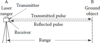
1. The first of these involves the accurate measurement of the TOF of a very short but intense pulse of laser radiation to travel from the laser ranger to the object being measured and to return to the instrument after having been reflected from the object—hence the use of the term pulse echo mentioned earlier. Thus, the laser ranging instrument measures the precise time interval that has elapsed between the pulse being emitted by the laser ranger located at point A and its return after reflection from a ground object located at point B (Figure 1.1).

FIGURE 1.1 Basic operation of a laser rangefinder that is using the timed pulse or TOF method.

$R=\frac{\upsilon \cdot t}{2}$

(1.1)

where:

R is the slant distance or range

υ is the speed of electromagnetic radiation, which is a known value

t is the measured time interval

From this, the following simple relationship can be derived:

$\Delta R=\frac{\Delta \upsilon .t}{2}+\frac{\upsilon .\Delta t}{2}$

(1.2)

where:

ΔR is the range precision

Δυ is the velocity precision

Δt is the corresponding precisio...

Table of contents

• Cover
• Half Title
• Title Page
• Copyright Page
• Table of Contents
• Preface to the Second Edition
• Preface to the First Edition
• Editors
• Contributors
• Chapter 1 Introduction to Laser Ranging, Profiling, and Scanning
• Chapter 2 Terrestrial Laser Scanners
• Chapter 3 Airborne and Spaceborne Laser Profilers and Scanners
• Chapter 4 LiDAR Systems and Calibration
• Chapter 5 Pulsed Laser Altimeter Ranging Techniques and Implications for Terrain Mapping
• Chapter 6 Georeferencing Component of LiDAR Systems
• Chapter 7 Full-Waveform Analysis for Pulsed Laser Systems
• Chapter 8 Strip Adjustment
• Chapter 9 Accuracy, Quality Assurance, and Quality Control of Light Detection and Ranging Mapping
• Chapter 10 Data Management of Light Detection and Ranging
• Chapter 11 LiDAR Data Filtering and Digital Terrain Model Generation
• Chapter 12 Forest Inventory Using Laser Scanning
• Chapter 13 Integration of LiDAR and Photogrammetric Data: Triangulation and Orthorectification
• Chapter 14 Feature Extraction from Light Detection and Ranging Data in Urban Areas
• Chapter 15 Global Solutions to Building Segmentation and Reconstruction
• Chapter 16 Building and Road Extraction from LiDAR Data
• Chapter 17 Progressive Modeling of 3D Building Rooftops from Airborne LiDAR and Imagery
• Chapter 18 A Framework for Automated Construction of Building Models from Airborne LiDAR Measurements
• Chapter 19 Quality of Buildings Extracted from Airborne Laser Scanning Data—Results of an Empirical Investigation on 3D Building Reconstruction
• Index