Using Microsoft Excel, the market leading spreadsheet package, this book combines theory with modelling aspects and spreadsheet analysis. Microeconomics Using Excel provides students with the tools with which to better understand microeconomic analysis.It focuses on solving microeconomic problems by integrating economic theory, policy analysis and
Trusted by 375,005 students
Access to over 1.5 million titles for a fair monthly price.
In Chapter 1 we discuss the basic concepts of supply, demand and price policies, and we formulate an appropriate Excel model. In order to do this, supply and demand functions are defined and the process of price formation on a market without and with government intervention is illustrated. We then discuss how various price policies affect political objectives such as producer revenue, consumer expenditure, foreign exchange or government budget.
Theory
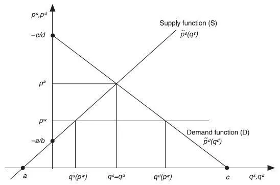
The starting point for the analysis of price policies on a market is the formulation of supply and demand functions. Let us consider the following linear supply function:
(1.1)
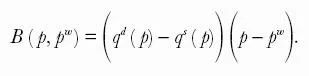
where qs(.) – supply function qs– quantity supplied ps– supply price.
Parameter a describes the hypothetical quantity of supply for a supply price of zero, and the value will be negative since supply will only begin above a certain minimum supply price. Parameter b describes the slope of the supply function and indicates the change in units supplied as a consequence of an increase of the supply price by one unit, exactly: by one infinitesimally small unit. It is common to graphically show supply and demand functions as inverse functions with the price on the y-axis and the quantity on the x-axis. Solving (1.1) with respect to ps yields the following inverse supply function:
(1.1)'
where
(.) – inverse supply function.
The function is visualised in Figure 1.1.
Similar to the supply side, the following linear demand function can be formulated:
(1.2)
where qd (.) – demand function qd – quantity demanded pd – demand price.
Parameter c marks a saturated situation. Parameter d is the slope of the demand function indicating the change in units demanded as a consequence of an increase of the demand price by one unit, exactly: by one infinitesimally small unit.
Solving (1.2) with respect to pd yields the following inverse demand function illustrated in Figure 1.1:
(1.2)'
where
(.) – inverse demand function.
Let us now consider a closed economy without government intervention. For such a policy framework there will be an equilibrium price on the market equalising supply and demand. This is the autarky price pa in Figure 1.1. Under free trade, instead, the world market price pw will be the relevant price for domestic supply and demand. We assume that the world market price is given for the domestic market; this is the ‘small country assumption’ according to which the world market price will not change due to domestic supply and demand changes. According to Figure 1.1, domestic supply and demand will be qs ( pw ) and qd ( pw ) under free trade and imports will be qim = qd ( pw ) – qs ( pw ). Autarky and free trade as discussed here mark the absence of government interventions in a market, but the scenarios may also be interpreted as describing only the specific policy framework: autarky and free trade.
Figure 1.1 Linear supply and demand functions.
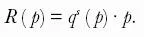
Let us now consider that a country sets the domestic price independently of the world market price according to domestic policy objectives. Such a price policy can be implemented by price and quantity interventions; in market economies the typical intervention is a ‘subsidisation’ or a ‘taxation’ of economic activities yielding domestic supply and/or demand prices different from the world market price. In Figure 1.2 a protectionist price policy is visualised that may be implemented by a tariff in an import situation or an export subsidy in an export situation. Formally, policy objectives on this market such as increasing producer revenue or government budget now depend on the world market price and/or the domestic price.
Figure 1.2 presents the case of a protectionist price policy in an import situation. As compared to free trade, the quantity of supply increases to qs ( p) and the quantity of demand decreases to qd ( p). Further relevant policy objectives may be defined for this protectionist price policy. The producer revenue will be:
(1.3)
Figure 1.2 Consequences of a protectionist price policy in an import situation.
For consumer expenditure we get:
(1.4)
In the import situation considered here import expenditures occur. In general, covering both an import and an export situation, we define a foreign exchange function as follows:
(1.5)
Thus, foreign exchange is a function of the two exogenous prices and it has a negative value in the import situation considered. Similarly, we define a government budget function:
(1.6)
The value of this function is positive for the case considered. It would be negative for a protectionist price policy in an export situation to be established by an export subsidy. Foreign exchange (expenditure) and government budget (revenue) are visualised in Figure 1.2.
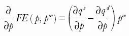
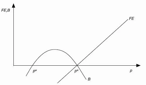
The values of the defined functions can now be calculated depending on the values of the exogenous prices and the parameters of the supply and demand functions. In order to assess the impact of the prices on these functions, it is helpful to draw the corresponding graphs of these functions. Foreign exchange will thus be a linear rising function of the domestic price p as the derivative of this function is a constant. It intersects the price axis at the autarky price pa. The foreign exchange function is visualised in Figure 1.3.
(1.5)'
Figure 1.3 also shows the government budget function with respect to the domestic price. For the linear supply and demand functions considered, we get a strictly concave quadratic budget function, intersecting the price axis at free trade p = pw and autarky at p = pa. At a domestic price level below the world market price, import subsidies are paid and, hence, budget expenditures occur that decrease with a rising domestic price. For a domestic price level between free trade pw and autarky pa, tariffs create budget revenues, with a maximum exactly between pw and pa. Finally, with higher domestic prices above the autarky price pa, increasing budget expenditures occur due to export subsidies.
Figure 1.3 Foreign exchange and government budget as a function of the domestic price.
Based on (1.5) and (1.6), analogous foreign exchange and government budget function...
Table of contents
Cover Page
Title Page
Copyright Page
Preface
Free Online Content Access Instructions
Symbols
Introduction
Part I: Analysis of Price Policies
Part II: Analysis of Structural Policies
Part III: Multi-Market Models
Part IV: Budget Policy and Priority Setting
Bibliography
Frequently asked questions
Yes, you can cancel anytime from the Subscription tab in your account settings on the Perlego website. Your subscription will stay active until the end of your current billing period. Learn how to cancel your subscription
No, books cannot be downloaded as external files, such as PDFs, for use outside of Perlego. However, you can download books within the Perlego app for offline reading on mobile or tablet. Learn how to download books offline
Perlego offers two plans: Essential and Complete
Essential is ideal for learners and professionals who enjoy exploring a wide range of subjects. Access the Essential Library with 800,000+ trusted titles and best-sellers across business, personal growth, and the humanities. Includes unlimited reading time and Standard Read Aloud voice.
Complete: Perfect for advanced learners and researchers needing full, unrestricted access. Unlock 1.5M+ books across hundreds of subjects, including academic and specialized titles. The Complete Plan also includes advanced features like Premium Read Aloud and Research Assistant.
Both plans are available with monthly, semester, or annual billing cycles.
We are an online textbook subscription service, where you can get access to an entire online library for less than the price of a single book per month. With over 1.5 million books across 990+ topics, we’ve got you covered! Learn about our mission
Look out for the read-aloud symbol on your next book to see if you can listen to it. The read-aloud tool reads text aloud for you, highlighting the text as it is being read. You can pause it, speed it up and slow it down. Learn more about Read Aloud
Yes! You can use the Perlego app on both iOS and Android devices to read anytime, anywhere — even offline. Perfect for commutes or when you’re on the go. Please note we cannot support devices running on iOS 13 and Android 7 or earlier. Learn more about using the app
Yes, you can access Microeconomics using Excel by Gerald Schwarz,Kurt Jechlitschka,Dieter Kirschke in PDF and/or ePUB format, as well as other popular books in Economics & Business General. We have over 1.5 million books available in our catalogue for you to explore.