Biological Processes in Living Systems

C. H. Waddington

• Publisher: Routledge
• Year: 2017
• ISBN:
  9781351297141
• Edition: 1
• Topic: Biological Sciences
• Subtopic: Biology
• Index: Biological Sciences

Biological Processes in Living Systems is the fourth and final volume of the Toward a Theoretical Biology series. It contains essays that deal in detail with particular biological processes: morphogenesis of pattern, the development of neuronal networks, evolutionary processes, and others. The main thrust of this volume brings relevance to the general underlying nature of living systems. Faced with trying to understand how the complexity of molecular microstates leads to the relative simplicity of phenome structures, Waddington-on behalf of his colleagues-stresses on the structure of language as a paradigm for a theory of general biology. This is language in an imperative mood: a set of symbols, organized by some form of generative grammar, making possible the conveyance of commands for action to produce effects on the surroundings of the emitting and the receiving entities. "Biology, " he writes, "is concerned with algorithm and program." Among the contributions in this volume are: "The Riemann-Hugoniot Catastrophe and van der Waals Equation, " David H. Fowler; "Differential Equations for the Heartbeat and Nerve Impulse, " E. Christopher Zeeman; "Structuralism and Biology, " Rene Thom; "The Concept of Positional Information and Pattern Formation, " Lewis Wolpert; "Pattern Formation in Fibroblast Cultures, " Tom Elsdale; "Form and Information, " C. H. Waddington; "Organizational Principles for Theoretical Neurophysiology, " Michael A. Arbib; "Stochastic Models of Neuroelectric Activity, " Jack D. Cowan. Biological Processes in Living Systems is a pioneering volume by recognized leaders in an ever-growing field.

Differential equations for the heartbeat and nerve impulse

E. C. Zeeman

University of Warwick

We abstract the main dynamical qualities of the heartbeat and nerve impulse, and then build the simplest mathematical models with these qualities. The results are flows on R² and R³. which are related to Thom’s cusp catastrophe [1–3]. In the case of the heart we explain how many of the complexities of the beat can be deduced from a simple behaviour of the muscle fibre. In the case of the nerve impulse we fit the model to the experimental data of Hodgkin and Huxley [4, 5]. The model provides an alternative to the latter’s own equations, and suggests alternative underlying chemistry.

In these two examples catastrophe theory provides not only a better conceptual understanding, by giving a single global picture that enables an overall grasp of the phenomenon, but also provides explicit equations for testing experimentally. The novelty of the approach lies in modelling the dynamics (which is relatively simple) rather than the biochemistry (which is relatively complicated). This approach might be useful for a large variety of phenomena in biology, whenever there is a trigger mechanism leading to some specific action. In an appendix we suggest how it might be applied to evolution.

Mathematically the equations that we derive are interesting, because they are generalizations of the Van der Pol and Lienard equations.

Part One

1.1. THREE QUALITIES

The three dynamic qualities displayed by heart muscle fibres and nerve axons are:

(1) stable equilibrium;

(2) threshold, for triggering an action;

(3) return to equilibrium.

The third quality can be divided into two cases according as to whether or not the return is smooth:

(3a) jump return (heart);

(3b) smooth return (nerve).

In the first half of the paper our objective will be to take these three qualities as ‘axioms’, and derive mathematical models by means of qualitative mathematical argument. We state the models in Theorems 1, 2 in sections 1.7 and 1.10 respectively, and apply them qualitatively to heart and nerve in sections 1.8 and 1.11. In order to keep the mathematics as translucent as possible, we only touch upon the physiology where necessary.

In the second half of the paper the models are developed quantitatively into a form that could be used for prediction, and for this we need to go more deeply into the physiology and numerical data. In sections 2.1 to 2.3 we discuss the heart, and in sections 2.4 to 2.10 the nerve, concluding both cases by suggesting how the models might be used in experiments. But first we must explain why we chose these three qualities.

There are two states to the heart, the diastole which is the relaxed state, and the systole which is the contracted state. If the heart stops beating it stays relaxed in diastole, which is therefore the stable equilibrium of Quality 1. What makes the heart contract into systole is a global electrochemical wave emanating from a pacemaker. As the wave reaches each individual muscle fibre, it triggers off the action of Quality 2, that makes the fibre rapidly contract. Each fibre remains contracted in the systole state for about 1/5 second, and then rapidly relaxes again—in other words the fibre obeys the jump return to equilibrium of Quality 3a. Therefore the three qualities describe the local behaviour for an individual muscle fibre, and our first objective is to describe this by an ordinary differential equation, which we achieve in Theorem 1. In section 2.1 we deal with the global structure of the heart and its four chambers, and in section 2.2 describe the pacemaker wave by a separate geodesic flow.

Now for the nerve impulse. A neuron, or nerve cell is in some ways like a tree (see Figure 1).

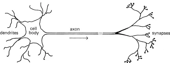
FIGURE 1

Corresponding to the roots of the tree are the dendrites, through which the neuron receives messages. Out of the cell body grows the axon, which is like the trunk of the tree. Just as the trunk of a tree divides into many branches, ending in thousands of leaves, so the axon divides into many branches, ending in thousands of synapses, which touch the dendrites of other neurons. It is the axons that connect up the whole nervous system, and comprise the white matter of our brains, while the dendrites and cell bodies comprise the grey matter. Messages travel along the axon to the synapses, and are thus transmitted to other neurons. This is the basic mechanism underlying the working of the brain, and so it is interesting to examine the nature of the message. A message consists of a series of spikes (see Figure 2).

Each spike is an electrochemical phenomenon that lasts about 1 msec (= 10^–3 sec), and travels very fast along the axon. The velocity is between 10 and 100 metres per second, depending upon the type of nerve. The simplest way to observe a spike is to put electrodes inside and outside the axon in order to measure the potential difference v of the inside relative to the outside, and then plot v against time (see Figure 3). While no message is passing the membrane surrounding the axon is polarized, and v remains constant about –65 mV (1 mV=10^–3 volts). This constant is called the resting potential, and represents the stable equilibrium of Quality 1. As the spike moves along the axon it triggers off a rapid depolarization of the membrane, called the action potential, which causes v to swing to +40 mV, representing the action of Quality 2. When the spike has passed, the membrane repolarizes relatively slowly, representing the smooth return to equilibrium of Quality 3b. These features can be seen in Figure 3, which is taken from Hodgkin [5, p. 64]. Notice that the potential V shown in Figure 3 is relative to the resting potential,

Therefore the resting potential is V = 0, while the maximum action potential is V = 115. This notation will be convenient later. The lower graph in Figure 3 is experiment, whilst the upper graph is given by the Hodgkin-Huxley model. The analogous graph given by our model is shown in Figure 26 below (see p. 60), with a calculated velocity of 21·9 m/sec.

As in the case of the heart muscle fibre, the three qualities represent the local behaviour at a single point of the axon, and our first objective will be to represent this by an ordinary differential equation in section 1.11. Later we shall incorporate into the model the global propagation wave by a partial differential equation; we shall find in section 2.8 Theorem 3 an explicit solution for the wave, and show how it triggers the local action. In section 2.4 we emphasize the importance of keeping the local and global ideas separate.

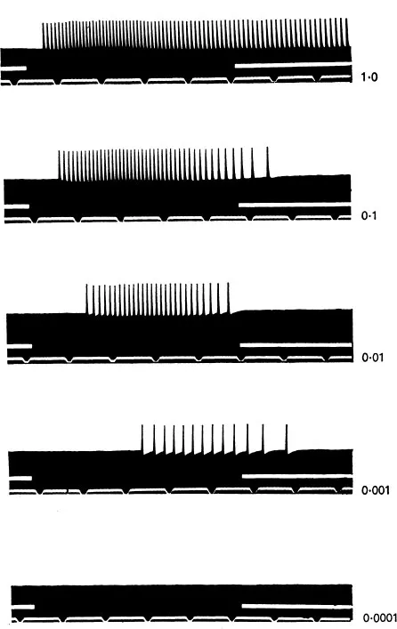
FIGURE 2
Impulses set up in optic nerve fibre of Lumulus by one second flash of light with relative intensities shown at right....

Table of contents

• Cover
• Half Title
• Title Page
• Copyright Page
• Table of Contents
• Preface
• The Riemann–Hugoniot catastrophe and van der Waals equation
• Differential equations for the heartbeat and nerve impulse
• Structuralism and biology
• The concept of positional information and pattern formation
• Pattern formation in fibroblast cultures, an inherently precise morphogenetic process
• Form and information
• Organizational principles for theoretical neurophysiology
• Stochastic models of neuroelectric activity
• Statistical and hierarchical aspects of biological organization
• The importance of molecular hierarchy in information processing
• What can we know about a metazoan’s entire control system ?: on Elsasser’s, and other epistemological problems in cell science
• Laws and constraints, symbols and languages
• Biology and meaning
• Appendix. A catastrophe machine
• Epilogue
• Indexes: Participants
• Author
• Subject