Statistics Explained

Perry R. Hinton

• Publisher: Routledge
• Year: 2014
• ISBN:
  9781317753919
• Edition: 3
• Topic: Psicología
• Subtopic: Historia y teoría en psicología

Statistics Explained is an accessible introduction to statistical concepts and ideas. It makes few assumptions about the reader's statistical knowledge, carefully explaining each step of the analysis and the logic behind it. The book:

• 
  
  

• provides a clear explanation of statistical analysis and the key statistical tests employed in analysing research data

• 
  
  

• gives accessible explanations of how and why statistical tests are used

• 
  
  

• includes a wide range of practical, easy-to-understand worked examples.

Building on the international success of earlier editions, this fully updated revision includes developments in statistical analysis, with new sections explaining concepts such as bootstrapping and structural equation modelling. A new chapter - 'Samples and Statistical Inference' - explains how data can be analysed in detail to examine its suitability for certain statistical tests.

The friendly and straightforward style of the text makes it accessible to all those new to statistics, as well as more experienced students requiring a concise guide. It is suitable for students and new researchers in disciplines including Psychology, Education, Sociology, Sports Science, Nursing, Communication, and Media and Business Studies.

Presented in full colour and with an updated, reader-friendly layout, this new edition also comes with a companion website featuring supplementary resources for students. Unobtrusive cross-referencing makes it the ideal companion to Perry R. Hinton's SPSS Explained, also published by Routledge.

Perry R. Hinton has many years of experience in teaching statistics to students from a wide range of disciplines and his understanding of the problems students face forms the basis of this book.

Introduction

1 ACCOMPANYING WEBSITE

 

To help us provide answers to research questions we collect data to advance our knowledge of the topic under study. There are a wide range of research methods and a broad definition of what can be called research data. It can range from the results of complex technological measuring devices (looking into, say, brain function or the formation of weather systems) to the way a political event is reported in media from different cultural groups or the descriptions people give of their friends or colleagues. Broadly speaking we distinguish between two types of data: quantitative and qualitative data. Quantitative data concerns numbers or quantities that we have collected using measuring devices such as timers, performance tests or questionnaires. Qualitative data concerns accounts, descriptions and explanations – often linguistic rather than numeric data. Most researchers focus on collecting either quantitative or qualitative data; and not surprisingly different analyses are performed on the two forms of data. This book is exclusively concerned with the former – quantitative data analysis – the analysis of numbers. Ultimately it is a combination of the two that will provide the fullest insight into our research questions. Consider research into the experience of students taking an examination. We might collect information on how many hours they spend studying, how many books they have read and how well they perform in the examination (quantitative data) but we might also ask them for their own explanations of how well they studied, accounts of their feelings and motivations, along with what they thought about the overall experience of taking the examination (qualitative data).

Quantitative data produces numbers. The numbers may be readily available such as the time it takes to perform a task, read off from a timer. But it may require some processing to produce the numbers: such as coding a questionnaire and entering or transferring the data to a suitable software application in order to produce the findings such as how many men and how many women answered ‘yes’ to question 4. Statistical analysis is a way of using these numbers to assist in answering research questions. Sometimes, but not often, it is possible to look at some research data and see what it is telling us, which we can then directly use to help form the answer to the research question. In this case we would not need to undertake any statistical analysis. Unfortunately, the implications of the data are rarely so obvious, especially when we have collected a large amount of data in numeric form. Simply looking at lots and lots of numbers is usually uninformative and possibly confusing. We need to draw from it the relevant information for the research question posed. This is where statistics can help us. A mass of data can be described and summarised or different sets of data can be compared by the calculation of appropriate statistics.

This book is about the logic and procedures of statistical analysis. Much of this book is about the calculation of various statistics. While we shall see in Chapter 5 that it has a technical definition, a statistic is essentially a way of describing a set of numbers. A ‘total’ is a statistic. We can find a total for the number of apples in a bowl or children in a school: we just add them up. Some statistics are easy to obtain (such as the number of fingers on my left hand) whereas others are a little more difficult to work out (such as the F-ratio in the analysis of variance – something we shall be looking at in Chapter 11). However, the purpose of calculating these statistics is to tell us something we want to know: can athletes run faster with a new design of shoe? which of two types of cola do people prefer? It is not the calculation of statistics that is intrinsically interesting but what the statistic tells us about the questions we are interested in. However, the ability to choose the appropriate statistic, and the ability to see whether our calculations are correct or not, are both crucial factors in obtaining a valid answer to our questions, rather than making an error: we don’t want to do the statistical equivalent of asking the time and being told it’s Tuesday. Enough detail is provided throughout the book so that most analyses can be worked through with the aid of a simple calculator, a spreadsheet application such as Excel or statistical software such as SPSS.

We invariably need to calculate statistics when we undertake certain forms of research and having an understanding of what they are and why we calculate them can make us much better able to critically analyse the work of others. If someone informs you that the statistical analysis of their research shows that pigs can fly, and people sometimes do make wild claims as a result of their research, then you might be sceptical about their choice or use of statistics. However, there are many cases where the claims are not so obviously in error yet a simple knowledge of statistical analysis can reveal a flaw.

The purpose of this book is to explain the logic behind statistical techniques, when you would use them and how you would calculate them. Often the latter tends to dominate one’s experience, and there is often a desire to just get the thing worked out, but it is understanding why one is calculating a particular statistic that is of crucial importance to data analysis.

The book begins with an explanation of the statistics that help us to describe data, examining what ‘frequency distributions’ can show us and which summary statistics we can calculate. It then moves on to the importance of the normal distribution and the logic of hypothesis testing, which uses probability values associated with the null hypothesis to make statistical judgements of ‘significance’. The difference between populations and samples is considered along with the use of information from samples to estimate the details of populations. The importance of sampling distributions to statistical analysis is explained. Subsequently various techniques are introduced that allow us to compare data from different samples.

The book can be read straight through to see the way in which the statistical tests have been developed. These tests all have a logical basis, and explanations are provided for the particular formulae that we use for our calculations. Alternatively, the book can be dipped in and out of, providing enough information on each test so that readers requiring a specific analysis can see why it has been developed and undertake an analysis on their own data by following the worked examples provided.

The rapid advances in computing power mean that data-crunching analyses can be undertaken such as bootstrapping and structural equation modelling using readily available statistical software applications such as SPSS (rather than by calculator or spreadsheet applications). Even though the full data analysis cannot be shown in detail for these complex analyses, enough information is provided to show how they are undertaken (such as in Chapter 22) and each of the techniques are explained so that the underlying logic of the test is clear.

The penultimate chapter provides an introduction to the model underlying many of our statistical tests. In the explanation of this model we can see why many statistical tests require a particular set of assumptions. While this chapter does not contain any new statistical techniques to learn it is hoped that the reader who does tackle this chapter will gain a deeper understanding of the principles underlying statistical techniques, which can lead to a greater appreciation of what in practice is happening when carrying out a statistical analysis.

ACCOMPANYING WEBSITE

This new edition also comes with a companion website featuring supplementary resources for students. Please go to www.routledge.com/cw/hinton for more details.

Descriptive statistics

2 MEASURES OF ‘CENTRAL TENDENCY’ MEASURES OF ‘SPREAD’ DESCRIBING A SET OF DATA: IN CONCLUSION COMPARING TWO SETS OF DATA WITH DESCRIPTIVE STATISTICS SOME IMPORTANT INFORMATION ABOUT NUMBERS CHAPTER RECAP

A major reason for calculating statistics is to describe and summarise a set of data. A mass of numbers is not usually very informative so we need to find ways of abstracting the key information that allows us to present the data in a clear and comprehensible form. In this chapter we shall be looking at an example of a collection of data and considering the best way of describing and summarising it.

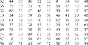
One hundred students sit an examination. After the examination the papers are marked and given a score out of one hundred. You are given the results and asked to present them to a committee that monitors examination performance. You are faced with the following marks:

Fortunately, you are told the sort of questions the committee might ask:

■ Can you describe the results of the examination?

■ Can you give us a brief summary of them?

■ What is the average mark?

■ What is the spread of scores?

■ What is the highest and lowest mark?

■ Here are last year’s results, how do this year’s compare?

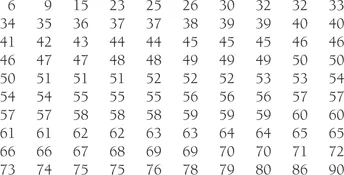
You sit looking at the above table. The answers to the questions are not obvious from the ‘raw’ data, that is, the original data before any statistics have been calculated. We need to do something to make it clearer. The first thing that we can do is to list the data in order, from lowest to highest:

With this ordering certain things are more apparent: we can now see the lowest and highest scores more easily, with the scores falling between 6 and 90.

Another thing we can do to improve our presentation is to add up the number of people who achieved the same mark. We work out the frequency of each mark. For example, 3 people scored 52 and only 1 scored 67. When we do this it allows us to see that the most ‘popular’ mark was 57 with a frequency of 4. We should not forget that there is a number of possible marks that no one achieved: no one scored 12 or 83 for example, so each of these marks has a frequency of 0.

frequency

The number of times a score, a range of scores, or a category is obtained in a set of data is referred to as its frequency.

We can present this information in graphical form if we convert it to a histogram, where the frequency of a mark is represented as a vertical bar. In the histogram, shown in Figure 2.1, we list out all the possible marks that a student could get, 0 to 100, and draw a bar above each mark, with the length of the bar corresponding to the frequency of the mark in the set of results. For a mark of 55 we draw a bar of length 3 (as 3 students obtained a mark of 55) and for 64 we draw a bar of length 2. This gives a clear visual presentation of the results.

histogram

A plot of data on a graph, where vertical bars are used to represent the frequency of the scores, range of scores or categories under study.

This histogram is called a frequency distribution, as we can see how the marks are distributed across t...

Table of contents

• Cover
• Half Title
• Title Page
• Copyright Page
• Dedication
• Table of Contents
• List of figures
• Preface
• Chapter 1 Introduction
• Chapter 2 Descriptive Statistics
• Chapter 3 Standard Scores
• Chapter 4 Introduction to Hypothesis Testing
• Chapter 5 Sampling
• Chapter 6 Hypothesis Testing with One Sample
• Chapter 7 Selecting Samples for Comparison
• Chapter 8 Hypothesis Testing with Two Samples
• Chapter 9 Significance, Error and Power
• Chapter 10 Samples and Statistical Inference
• Chapter 11 Introduction to the Analysis of Variance
• Chapter 12 One Factor Independent ANOVA
• Chapter 13 Multiple Comparisons
• Chapter 14 One Factor Repeated Measures ANOVA
• Chapter 15 The Interaction of Factors in the Analysis of Variance
• Chapter 16 The Two Factor ANOVA
• Chapter 17 Two Sample Nonparametric Analysis
• Chapter 18 One Factor ANOVA for Ranked Data
• Chapter 19 Analysing Frequency Data: Chi-Square
• Chapter 20 Linear Correlation and Regression
• Chapter 21 Multiple Correlation and Regression
• Chapter 22 Complex Analyses
• Chapter 23 An Introduction to the General Linear Model
• Chapter 24 Postscript
• Appendix: Acknowledgements and Statistical Tables
• Glossary
• References
• Index
• Choosing a statistical test