Computational Economics

A concise introduction

Oscar Afonso, Paulo B. Vasconcelos

• Publisher: Taylor & Francis
• Year: 2015
• eBook ISBN: 9781317508656
• Edition: 1
• Topic: Business
• Subtopic: Business General
• Index: Business

Computational Economics: A concise introduction is a comprehensive textbook designed to help students move from the traditional and comparative static analysis of economic models, to a modern and dynamic computational study. The ability to equate an economic problem, to formulate it into a mathematical model and to solve it computationally is becoming a crucial and distinctive competence for most economists.

This vital textbook is organized around static and dynamic models, covering both macro and microeconomic topics, exploring the numerical techniques required to solve those models.

A key aim of the book is to enable students to develop the ability to modify the models themselves so that, using the MATLAB/Octave codes provided on the book and on the website, students can demonstrate a complete understanding of computational methods.

This textbook is innovative, easy to read and highly focused, providing students of economics with the skills needed to understand the essentials of using numerical methods to solve economic problems. It also provides more technical readers with an easy way to cope with economics through modelling and simulation. Later in the book, more elaborate economic models and advanced numerical methods are introduced which will prove valuable to those in more advanced study.

This book is ideal for all students of economics, mathematics, computer science and engineering taking classes on Computational or Numerical Economics.

Part I
Static economic models

1
Supply and demand model

Introduction

In microeconomics, the supply–demand model is required to understand the determination of the price and of the quantity of a good sold on the market. The mechanism depends on the interaction of two different groups: buyers and sellers. The model assumes a high degree of competition, meaning that there are many buyers and sellers in the market for bidding to take place. Buyers bid against each other and thereby raise the price, and sellers bid against each other and thereby lower the price. The equilibrium is a point at which all the bidding has been done and nobody has an incentive to offer higher prices or accept lower prices. This is a partial equilibrium because it ignores the connections between markets and only studies the way individual markets work.

The assumed perfect competition assumption is an abstraction, because no market is actually perfectly competitive, but the framework still provides a good approximation for what is happening much of the time. Thus, the model, initially approached by Smith (1776), Ricardo (1817) and Cournot (1838), is simplified to regard the quantity demanded and the quantity supplied as functions of the price of the goods. The standard graphical representation, usually attributed to Marshall (1890), has price on the vertical axis and quantity on the horizontal axis. Since determinants of demand and supply other than the price of the goods in question are not explicitly represented, changes in the values of these variables are represented by moving the supply and demand curves. In turn, responses to changes in the price of the good are represented as movements along unchanged demand and supply curves.

This model is defined in a closed economy. It is then extended to an open context to accommodate international trade policy, by considering tariffs to imports and subsidies to exports. The market effects as well as social welfare effects are analysed.

In this chapter, the model is described by a system of linear equations (for a nonlinear version, see Appendix A). The solution provides the market equilibrium price and quantity. With an automatic procedure, it is straightforward to evaluate the impacts of changes in some exogenous factors that affect demand or supply and, also, to measure those impacts on social welfare.

The description of the economic model follows Varian (1992, ch. 1, 3, 9–10), Perloff (2013, ch. 1–5), Mas-Colell et al. (1995, part I) and Krugman et al. (2011, part II). In turn, the numerical methods are explained according to Golub and Van Loan (1996, ch. 3), Demmel (1997, ch. 2) and Dahlquist and Björck (2008, ch. 1).

Economic model in autarky

Variables, parameters and functional forms

As in any model, the supply–demand model is composed of endogenous and exogenous variables, parameters and functional forms, which link variables and parameters.

The standard equations that characterise the economy are:

• demand,
  
  ;
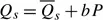
• supply,
  
  .

The endogenous variables are: quantity demanded, Q_d; quantity offered, Q_s; price of the good, P.

The exogenous variables are: independent/autonomous quantity demanded,

; independent/autonomous quantity offered,

.

In the functional forms above, a and b are parameters: a > 0 is the sensitivity of the demand to price and b > 0 is the sensitivity of the supply to price.

Demand

Quantity demanded, Q_d, is the total amount of a good (or of a service) that buyers would choose to purchase under given conditions, which include the price of the good, P, as well as other variables, represented by the exogenous variable

, such as income and wealth, prices of substitutes and complements, population, preferences (tastes) and expectations of future prices. That is, all of these things are considered, with the exception of the price of the good, as determinants of demand. Indeed, when we refer to the demand, we are focusing on the relationship between quantity demanded and price (while holding all the others fixed).

The Law of Demand states that when the price of a good rises,...

Table of contents

• Cover
• Title
• Copyright
• Contents
• List of figures
• Preface
• Using the book
• Introduction
• PART I Static economic models
• PART II Dynamic economic models
• PART III Appendices
• Bibliography
• Index