Distributed Sensor Arrays

Localization

Prabhakar S. Naidu

• Publisher: CRC Press
• Year: 2017
• ISBN:
  9781351792837
• Edition: 1
• Topic: Technology & Engineering
• Subtopic: Electrical Engineering & Telecommunications
• Index: Technology & Engineering

Localization of transmitters and receiving sensors is achieved by measuring radiation emitted by a source to a set of sensors, which are either on a definite pattern, known as an array, or one randomly located at irregular points, known as a distributed sensor array. This book discusses how to determine the position of sensors and transmit information to a central node, also known as the anchor node. Time of arrival, time difference of arrival, frequency time of arrival, and strength of received signal are also covered. The reader will learn effective algorithms and implementation, as well as numerical examples, with the inclusion of lab experiments. It discusses time synchronization, including the rotating laser beam to measure distance, in detail.

1	Distributed Sensor Arrays

There are many engineering applications where it is difficult to build a regular array because of practical limitations, in the case of a forest fire or for flood control, for example. During war, to monitor enemy troop movement, wireless sensors are often used by projecting them into enemy territory. In such a situation, it is impossible to build a regular sensor array. Likewise, in wireless communications, non-invasive localization of a tumor in biomedical investigation, when tracking a moving vehicle, leakage of crude oil from a pipeline, or in seismic exploration for hydro-carbons, placement of sensors is often constrained by the accessible space.

This chapter explores different localization techniques where the sensors are randomly distributed. Since time synchronization is a difficult task in distributed sensor arrays (DSAs), we emphasize methods that do not require time synchronization. Toward this end, we provide details of localization methods based on received signal strength, lighthouse effect, frequency difference of arrival (FDoA) measurements, and phase difference estimation.

DSAs are considered wired when all sensors are connected to a central processor, either through physical wire or microwave communication (wireless). In the first category, we have a regularly shaped array, for example, linear, rectangular, or circular arrays of known geometry. There are irregularly distributed but wired sensors; for example, randomly distributed sensors at known locations, connected to a central processor. When the array is very large and is populated with many tiny sensors with limited power source, it is no longer possible for sensors to individually communicate to the central processor. Either a sensor communicates with its nearest neighbor or at utmost with a local processor, also known as an anchor. But the sensor position is generally not known. Such a sensor array is known as an ad hoc array. In this chapter, we shall consider the response functions of various types of sensor distributions.

1.1REGULAR SENSOR ARRAY

A standard sensor array is a linear, rectangular, or circular array with equispaced sensors. There are variations of these geometries devised for specific applications, such as an L-shaped array in seismic monitoring or a towed array for naval applications.

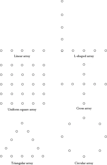
Some examples of regular planar array of sensors are shown in Figure 1.1. An important requirement is that the sensor spacing and the geometry of the array must be precisely controlled. Phase difference between successive sensors must be constant and its magnitude must be less than π. This requires the sensor spacing to be less than half-wavelength, λ/2 (except for circular array [1]). Random errors in the sensor spacing can result in large side lobes in the array response. Similarly, individual sensor response, required for defining the steering vector, must be carefully estimated. This is known as array calibration. These are some of the nagging problems faced by any sensor array designer. These issues have been discussed in an earlier companion publication [2]. In the present work, we relax some of these stringent requirements. The sensors are no longer required to be arranged in any specific order. Often, we have many redundant sensors, allowing a kind of trade-off between a precisely controlled array of a small number of sensors versus an array of a large number of randomly placed sensors.

FIGURE 1.1Some examples of regular planar arrays.

1.2WIRED SENSOR ARRAY

In many applications, it is not possible to achieve an ordered distribution of sensors, particularly when we have a very large number of sensors over a large area. But the location of sensors is precisely known. A recent example of such a large array is the largest radio telescope in the world, consisting of 25,000 small antennas distributed over Western Europe (aperture ≈ 1000 km). Sometimes, the constraints of space, for example in biomedical applications, demand sensors to be distributed over available space. In a distributed array of the previously mentioned type, all sensors are wired (or alternatively connected wirelessly) to a central processing unit where most of the signal processing tasks are carried out. Sensors, however, perform signal conditioning, A/D conversion, and so on. Each sensor is also able to communicate with the central processor. The location of all sensors is known, but the location of the transmitter and the emitted signal waveform are unknown. Wired sensor arrays of this type are usually small, with a limited number of sensors strategically placed surrounding a target of interest. Sometimes it becomes necessary to keep the target away from the sensor array for safety or security reasons. Location estimation is based on ToA information at each sensor. ToA estimation requires the transmitter to send out a known waveform at a fixed time instant. The time of arrival at each sensor is measured relative to the instant of transmission. The clocks of all sensors and the clock at transmitter must be synchronized to get correct ToA estimates. In addition, the transmitter must be a friendly one so that it may be programmed to transmit a waveform at a preprogrammed time instant. When this is not possible (e.g., with an enemy transmitter), we can use TDoA at all pairs of sensors whose clocks are synchronized. One advantage of using of ToA or TDoA for localization is that it is not necessary to maintain λ/2 spacing between sensors as in a regular array. Nor is it necessary to calibrate sensors.

When a sensor is not equipped to estimate ToA/TDoA, the received signal would be sent to the central processing unit, which will then take over the tasks of ToA/TDoA estimation and target localization. In this case, the ToA/TDoA will include the time of communication from the sensor to the central processing unit. As the distance between each sensor and the central processing unit (anchor) is known, it is easy to estimate this communication time and subtract it from the measured ToA. This correction, however, is insignificant when we are dealing with acoustic or seismic arrays—as the speed of a sound wave is much lower than that of electromagnetic waves—used for communication from a sensor to the central processing unit.

1.2.1DSA RESPONSE

As in a regular sensor array, we can think of directivity or the beam pattern of a DSA. In a simple delay-and-sum beam formation, the outputs of all sensors, after suitable delay, are summed up to estimate the signal emanating from the chosen test point. Such a beam is also known as a focused beam [2]. The output power in the beam will represent a measure of our ability to detect the presence of a transmitter at the focal point. Thus, we can compute the array response at each point of space in the region of interest around the sensors. A large power peak at some point reve...

Table of contents

• Cover
• Half-Title
• Title
• Copyright
• Dedication
• Contents
• Preface
• Acknowledgements
• Author
• Chapter 1 Distributed Sensor Arrays
• Chapter 2 Basic Inputs
• Chapter 3 Estimation of ToA/TDoA/FDoA
• Chapter 4 Localization
• Chapter 5 Hybrid Methods for Localization
• Chapter 6 Self-Localization
• Index