Applied Power Analysis for the Behavioral Sciences

2nd Edition

Christopher L. Aberson

• Publisher: Routledge
• Year: 2019
• ISBN:
  9781351695053
• Edition: 2
• Topic: Psychology
• Subtopic: Research & Methodology in Psychology
• Index: Psychology

Applied Power Analysis for the Behavioral Sciences is a practical "how-to" guide to conducting statistical power analyses for psychology and related fields. The book provides a guide to conducting analyses that is appropriate for researchers and students, including those with limited quantitative backgrounds. With practical use in mind, the text provides detailed coverage of topics such as how to estimate expected effect sizes and power analyses for complex designs. The topical coverage of the text, an applied approach, in-depth coverage of popular statistical procedures, and a focus on conducting analyses using R make the text a unique contribution to the power literature. To facilitate application and usability, the text includes ready-to-use R code developed for the text. An accompanying R package called pwr2ppl (available at https://github.com/chrisaberson/pwr2ppl) provides tools for conducting power analyses across each topic covered in the text.

1

WHAT IS POWER?

Why is Power Important?

This chapter reviews null hypothesis significance (NHST) testing, introduces effect sizes and factors that influence power, discusses the importance of power in design, presents an introduction to noncentral distributions, addresses misconceptions about power, discusses typical levels of power in published work, examines strategies for determining an appropriate effect size for power analysis, critiques post hoc power analyses, and discusses typical levels of power used for design.

Review of Null Hypothesis Significance Testing

NHST focuses on conditional probabilities. The conditional probabilities used in NHST procedures address how likely it is to obtain an observed (i.e., sample) result given a specific assumption about the population. Formally, the assumption about the population is called the null hypothesis (e.g., the population mean is 0) and the observed result is what the sample produces (e.g., a sample mean of 10). Statistical tests such as z, χ², t, and Analysis of Variance (ANOVA) determine how likely the sample result or any result more distant from the null hypothesis would be if the null hypothesis were true. This probability is then compared to a set criterion. For example, if a result this far or farther from the null hypothesis would occur less than 5% of the time when the null is true, then we will reject the null. More formally, the criterion is termed a Type I or α error rate (5% corresponds to α = .05).

Table 1.1, common to most introductory statistical texts, summarizes decisions about null hypotheses and compares them to what is true for the data (“reality”). Two errors exist. A Type I or α error reflects rejecting a true null hypothesis. Researchers control this probability by setting a value for it (e.g., use a two-tailed test with α = .05). Type II or β errors reflect failure to reject a false null hypothesis. Controlling this probability is at the core of this book. Type II errors are far more difficult to control than Type I errors. Table 1.1 also represents correct decisions, either failing to reject a true null hypothesis or rejecting a false null. The probability of rejecting a false null hypothesis is power. As suggested by the title of this book, this topic receives considerable coverage throughout the text.

For power analysis, the focus is on situations for which the expectation is that the null hypothesis is false (see Chapter 10 for a discussion of approaches to “supporting” null hypotheses). Power analysis addresses the ability to reject the null hypothesis when it is false.

Effect Sizes and Their Interpretation

One of the most important statistics for power analysis is the effect size. Significance tests tell us only whether an effect is present. Effect sizes tell us how strong or weak the observed effect is.

Although researchers increasingly present effect size alongside NHST results, it is important to recognize that the term “effect size” refers to many different measures. The interpretation of an effect size is dependent on the specific effect size statistic presented. For example, a value of 0.14 would be relatively small in discussing the d statistic but large when discussing η². For this reason, it is important to be explicit when presenting effect sizes. Always reference the value (d, r, η², etc.) rather than just noting “effect size.”

TABLE 1.1 Reality vs. Statistical Decisions

Reality
		Null Hypothesis True	Null Hypothesis False
Research Decision	Fail to Reject Null	Correct failure to reject null 1–α	Type II or β error
Reject Null	Type I or α error	Correct rejection of null 1–β

TABLE 1.2 Measures of Effect Size, Their Use, and a Rough Guide to Interpretation

Effect Size	Common Use/Presentation	Small	Medium	Large
Φ (also known as V or w)	Omnibus effect for χ^2	0.10	0.30	0.50
h	Comparing proportions	0.20	0.50	0.80
d	Comparing two means	0.20	0.50	0.80
r	Correlation	0.10	0.30	0.50
q	Comparing two correlations	0.10	0.30	0.50
f	Omnibus effect for ANOVA/Regression	0.10	0.25	0.40
η^2	Omnibus effect for ANOVA	0.01	0.06	0.14
f ^2	Omnibus effect for ANOVA/Regression	0.02	0.15	0.35
R^2	Omnibus effect for Regression	0.02	0.13	0.26

Table 1.2 provides a brief summary of common effect size measures and definitions of small, medium, and large values for each (Cohen, 1992). Please note that the small, medium, and large labels facilitate comparison across effects. These values do not indicate the practical importance of effects.

What Influences Power?

I learned an acronym in graduate school that I use to teach about influences on power. That acronym is BEAN, standing for Beta (β), Effect Size (E), Alpha (α), and Sample Size (N). We can specify any three of these values and calculate the fourth. Power analysis often involves specifying α, effect size, and Beta to find sample size.

Power is 1–β. As α becomes more liberal (e.g., moving from .01 to .05), power increases. As effect sizes increase (e.g., the mean is further from the null value relative to the standard deviation), power increases. As sample size rises, power increases.

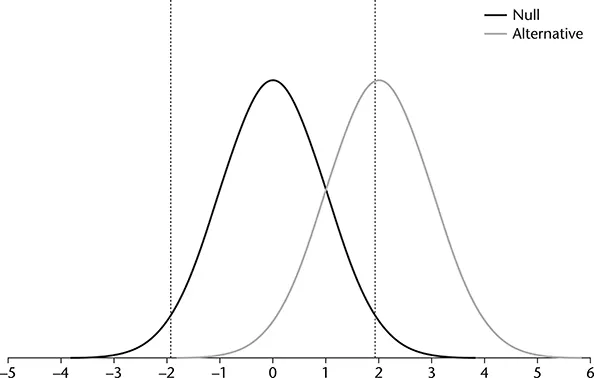
Several figures represent the influence of effect size, α, and sample size on power. Figure 1.1 presents two distributions: the null and the alternative. The null distribution is the distribution specified in the null hypothesis and represented on the left hand side of the graph. For this example, the null hypothesis is that the population mean is zero. The null sampling distribution of the mean is centered on zero, reflecting this null hypothesis. The alternative sampling distribution, found on the right hand side of each graph, reflects the distribution of means from which we are actually sampling. Several additional figures follow and are useful for comparison with Figure 1.1. For simplicity, the population standard deviation and the null hypothesis remain constant for each figure. For each of the figures, the lines represent the z_critical values.

FIGURE 1.1 Null and Alternative Distributions for a Two-Tailed Test and α = .05.

A sample mean allows for rejection of the null hypothesis if it falls outside the critical values that we set based on the null distribution. The vertical lines in Figure 1.1 represent the critical values that cut off 2.5% in each tail of the null distribution (i.e., a two-tailed test with α = .05). A little more than half of samples drawn from the alternative distribution fall above the upper critical value (the area to the right of the line near +2.0). Sample means that fall above the critical value allow for rejection of the null hypothesis. That area reflects the power of the test, about .50 in this example.

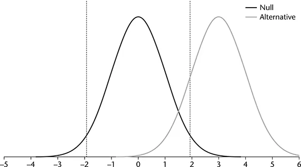
Now compare the power in Figure 1.1 to power in Figure 1.2. The difference between the situations represented in these two figures is that the effect size, represented in terms of the difference between the null and alternative means, is larger for Figure 1.2 than Figure 1.1 (recall that standard deviation is constant for both situations). The second figure shows that as the effect size increases, the distributions are further apart, and power increases because more of the alternative distribution falls in the rejection region.

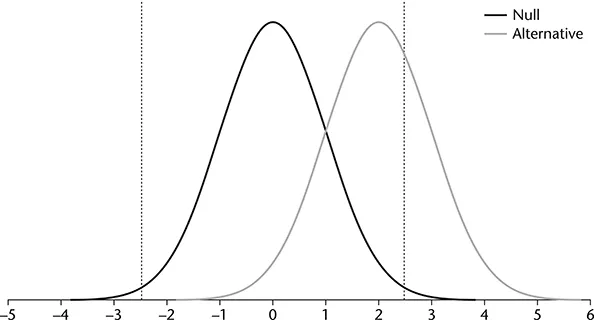
Next, we consider the influence of α on power. Figures 1.1 and 1.2 presented a two-tailed test with α = .05. Figure 1.3 reduces α = .01. Notice the change in the location of the vertical lines representing the critical values for rejection of the null hypothesis. Comparing Figures 1.1 and 1.3 shows that reducing α decreases power. The area in the alternative distribution that falls within the rejection region is smaller for Figure 1.3 than 1.1. Smaller values for α make it more difficult to reject the null hypothesis. When it is more difficult to reject the null hypothesis, power decreases.

FIGURE 1.2 Null and Alternative Distributions for a Two-Tailed Test With Increased Effect Size and α = .05.

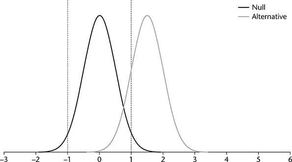
Figure 1.4 demonstrates the influence of a larger sample size on power. This figure presents distributions that are less disperse than those in Figure 1.1. For this figure, the x-axis represents raw scores rather than z-values. Recall from the Central Limit Theorem that the dispersion of a distribution of sample means (standard error of the mean) is a function of the standard deviation in the population and the sample size. Specifically, this is the standard deviation divided by the square root of sample size. As sample size rises, dispersion decreases. As seen in Figure 1.4 (assuming that the difference between the means of the distributions are the same for Figures 1.1 and 1.4), the reduced dispersion that results from larger samples increases power.

FIGURE 1.3 Null and Alternative Distributions for a Two-Tailed Test with α = .01.

FIGURE 1.4 Null and Alternative Distributions for a Two-Tailed Test and α = .05 with a Large Sample.

For an interactive tutorial on the topic, see the WISE (Web Interface for Statistics Education) home page at wise.cgu.edu. The web page includes a detailed interactive applet and tutorial on power analysis (see Aberson, Berger, Healy, & Romero, 2002 for a description and evaluation of the tutorial assignment). Chapters 2 and 3, particularly the material relevant to Figures 2.1 and 3.1, provide descriptions useful for power calculations.

Central and Noncentral Distributions

The examples presented in the preceding section use the normal distribution. In practice, these tests are less common in most fields than those conducted using t, F, or χ². Power analyses become more complex when using these distributions. Power calculations are based on the alternative distribution. When we use a z-test with a normally distributed null distribution, the alternative distribution is also normally distributed no matter the size of the effect. Distributions of this type are termed central distributions. However, when we d...

Table of contents

• Cover
• Half Title
• Title Page
• Copyright Page
• Table of Contents
• List of Figures
• List of Tables
• Preface
• Acknowledgments
• 1 What is Power? Why is Power Important?
• 2 Chi Square and Tests for Proportions
• 3 Independent Samples and Paired t-tests
• 4 Correlations and Differences between Correlations
• 5 Between Subjects ANOVA (One and Two Factors)
• 6 Within Subjects Designs with ANOVA and Linear Mixed Models
• 7 Mixed Model ANOVA and Multivariate ANOVA
• 8 Multiple Regression
• 9 Analysis of Covariance, Moderated Regression, Logistic Regression, and Mediation
• 10 Precision Analysis for Confidence Intervals
• 11 Additional Issues and Resources
• References
• Index