Higher Electronics

Mike James

• Publisher: Routledge
• Year: 2013
• ISBN:
  9781135389413
• Edition: 1
• Topic: Tecnología e ingeniería
• Subtopic: Ingeniería eléctrica y telecomunicaciones

Higher Electronics is a comprehensive text for electronics undergraduates, covering analogue, digital electronics and microelectronics in a single volume - at a level suitable for most first and second year modules. The text is highly student-centred, providing numerous
· worked examples with step-by-step guidance and hints
· highlighted key facts and points of interest
· self-check questions scattered through the text
· problem sections (with answers supplied)
It has been written to suit courses with an intake from a range of educational backgrounds, and a minimum of prior knowledge is assumed.
Higher Electronics has been written to be fully in line with units 8-12 of the new BTEC Higher National specifications from Edexcel. This makes it the text of choice for all students following an electronics / electrical pathway through an HNC or HND. The student-centred text is ideal for the new course, and follows on especially well for students from a GNVQ background. The style and approach of Higher Electronics is consistent with the new text from Newnes, Higher National Engineering, which covers the mandatory units (units 1-7) of the new Higher National scheme.

1	Power supplies

Summary

This chapter deals with the problem of providing stable, smooth dx. supplies that provide a constant voltage or current output The technologies described cover the range of those in common use – linear, switch-mode, step-down, step-up, with limiting or foldback.

1.1 Rectification and smoothing

This section deals with the conversion of a.c. mains electricity into a low voltage d.c. supply. Later sections will deal with the design of precision d.c. regulators which provide an accurate, overcurrent-protected, voltage source.

The first step is to reduce the mains supply to a lower a.c. equivalent. A transformer is used for this purpose. The a.c. high voltage is connected to the primary windings while the lower a.c. output is available from the secondary windings. Figure 1.1.1 shows three possible configurations which are commonly available off the shelf. Most commercial equipment has to work at European and American a.c. transmission voltages, hence the variety of primary windings. Europe requires 230 V @ 50 Hz, while the USA requires 110 V @ 60 Hz.

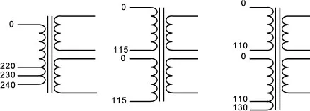
Figure 1.1.1 Transformer configurations

The transformer core is made from steel laminations. It supports the primary and secondary windings and guides the magnetic flux which links them. At the frequencies of 50 Hz and 60 Hz, laminated cores provide the best cost/efficiency compromise. The two frequencies are close enough so that no modifications are needed to enable the transformer to operate with either.

Table 1.1.1

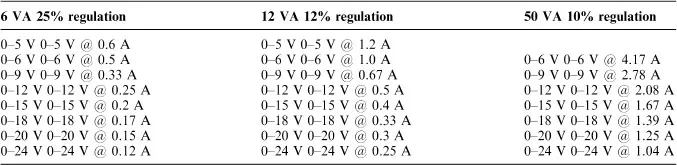
Data: Farnell Electronic Components Ltd

There are usually two secondary windings. These can either be left separate, connected in series for a higher output voltage or connected in parallel to obtain a higher current.

Power rating

The transformer must also be able to deliver sufficient current for the job in hand. Transformers are rated in volt-amperes (VA), which are a measure of the amount of real power they can handle. Table 1.1.1 shows a typical list of mains transformers and their ratings.

The lower the power handling, the worse is the percentage regulation. This is a measure of output voltage drop which will be explained and allowed for in the next section. A ‘dual 0-12 V 6VA’ transformer has two 0-12 V secondaries each capable of delivering 3 VA/12V = 0.25 A. These could deliver a total of:

24 V @ 0.25 A or 12 V @ 0.5 A or 2 × l2V @ 0.25A

Problems 1.1.1

What current is each secondary of the following transformers capable of delivering;

(1) dual 0-6 V 12VA;

(2) dual 0-9 V 25 VA;

(3) dual 0-12 V 50 VA?

RMS quantities

Each of the three waveforms has the same peak amplitude and the same frequency. Which of these three do you think is capable of delivering the most power to a load? For instance, which waveform would light a lamp to the brightest extent?

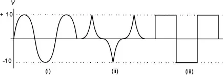
Figure 1.1.2 Voltage waveforms

The amplitude is characterized by assigning an amplitude quantity called F_RMS to it. RMS stands for ‘root mean square’ and it describes the mathematical process by which the voltage is calculated. For the waveforms above:

V_RMS(i) = 7.07 V; V_RMS (ii) = 2.00 V; V_RMS (iii) = 10.00 V

The power delivered by each of these three is given by:

Since a.c. is generated as a sine wave, then this is the figure which is most relevant. For a sine wave, it is fairly easy to prove that:

Mathematics in action

All of these waveforms are symmetrical, so their average value over one cycle will be zero. However, when you square a negative number, the answer is positive: for example, -2 × -2 = +4. This is the basis of calculating the root mean square. For any periodic waveform:

Square the value at all instants Find the mean value

Take the root of this mean of the squares.

Hence root-mean-square.

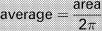
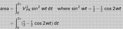
When a sine wave has a value of v = v_PK sin wt the square is v² = V²_pk sin² wt The mean value over one period is found by integrating the expression with respect to time from the range 0 to 2π. This gives the area under the square of the waveform. The average is then:

Working through this:

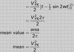
The root of the mean of the squares is thus:

Problems 1.1.2

(1) Calculate the peak voltage and the peak-peak voltage of the UK 230 V_RMS mains supply.

(2) What is the peak voltage to be expected from the secondary of a:

(a) 12 V mains transformer

(b) 15 V mains transformer

(transformer voltages are always quoted as RMS values).

Regulation

All real transformers exhibit a property called regulation. In a 12 V, 0.5 A secondary, the secondary will only output 12 V when it is actually delivering 0.5 A. At values of current less than this, the RMS voltage output will be higher, as shown in Figure 1.1.3.

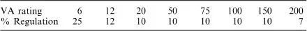
When zero current is drawn from the transformer, the secondary voltage rises to 13.44 V (in this case). The figure of 13.44 V comes from the fact that different VA ratings of transformers have the typical regulation figures shown in Table 1.1.2.

Table 1.1.2

Data: Farnell Electronic Components Ltd

So, from Tables 1.1.1 and 1.1.2, for a 12 VA transformer, the no-load secondary RMS voltage would be 12% higher or 13.44 V as shown. This effect is fairly linear, so a load of 0.25 A would result in a secondary voltage of 12.72 V.

Figure 1.1.3 Output voltage/ current characteristic of a transformer

There is a general rule that the smaller the transformer, the less magnetically efficient it is and so the worse the regulation. The leakage flux does not provide perfect linkage between primary and secondary windings. Another factor is the I²R losses which increase as the wire sizes get smaller. For example, the miniature encapsulated transformer range has the figures shown in Table 1.1.3.

Table 1.1.3

Data: Farnell Electronic Components Ltd

(1) (a) What is the no-load secondary voltage of a practical 15V, 4VA encapsulated transformer as in Table 1.1.3?

(b) What would the secondary voltage be when delivering 100 mA?

(2) What is the secondary terminal voltage of a 9 V, 6VA transformer delivering 250 mA? (Use data from Table 1.1.1)

Rectification

The next step is to convert the alternating voltage into a unidirectional voltage. Rectifier diodes are used for this.

Figure 1.1.4 A half wave rectifier

Figure 1.1.5 A full wave rectifier

Only one diode is needed for a half wave rectifier. When the output is positive, the diode conducts. When the voltage reverses, the diode blocks the current to produce the waveform shown. However, because silicon diodes are so cheap, it is rarely worth using this inefficient method. Full wave rectification can be achieved by one of two methods (Figures 1.1.5 and 1.1.6).

Diodes X and Y alternately conduct as secondary terminals A and D change polarity every half cycle. The load voltage will be (V_AB × – 0.6 V) or (V_CD × – 0.6 V) depending on the mains polarity at the time.

(V_AB × \fl) and (V_CD × \fl) is the peak output; 0.6 V is the forward voltage drop across each diode as it conducts.

Example 1.1.1

Calculate the peak load voltage of an ideal (regulation-less) 12V transformer.

Peak secondary voltage = 12 ×

= 17 V

Peak load voltage = 17 V – 0.6 V

= 16.4 V

Problems 1.1.4

(1) Calculate the peak load voltage of a rectified ideal 9 V transformer.

(2) Calculate the peak load voltage of a rectified 2VA 0-6/0-6 transformer when delivering 200 mA.

(3) What is the maximum d.c. voltage expected from a rectified 15V 50 VA transformer?

Figure 1.1.6 A full wave rectifier bridge

Figure 1.1.7 Typical bridge rectifier packages

Rectifier bridge

One of the most common configurations used for full wave rectifying an a.c. waveform is the rectifier bridge. Note that the direction of the diodes Dl and D2 point up to the +d.c. while D3 and D4 point away from the —d.c. (Figure 1.1.6). The diodes conduct in pairs:

Whe...

Table of contents

• Cover Page
• Title page
• Copyright page
• Contents
• Introduction
• 1 Power supplies
• 2 Feedback (1)
• 3 Power amplifiers
• 4 Feedback (2)
• 5 Operational amplifiers (1)
• 6 Noise
• 7 Operational amplifiers (2)
• 8 Oscillators
• 9 Radio frequency and other techniques
• 10 Logic circuits
• 11 Sequential logic
• 12 Microprocessors
• Appendix A Number systems
• Appendix B MCS51 Instruction set
• Index