Exploring Chaos

Theory And Experiment

Brian Davies

• Publisher: CRC Press
• Year: 2018
• ISBN:
  9780429982491
• Edition: 1
• Topic: Mathematics
• Subtopic: Mathematics General
• Index: Mathematics

This book presents elements of the theory of chaos in dynamical systems in a framework of theoretical understanding coupled with numerical and graphical experimentation. It describes the theory of fractals, focusing on the importance of scaling and ordinary differential equations.

Chapter 1

Introduction

1.1 Dynamical models

To the Greeks, chaos signified the infinite formless space which existed before the universe was created. To the generations of thinkers, philosophers and scientists of the succeeding ages, chaos and formlessness have been the subject of countless assaults in an extraordinary search for understanding of the world in which we live.

In the physical sciences these endeavours have been so successful that we can predict the motion of a space craft so as to enable it to be within a few kilometers of a chosen destination after a journey of several years. This level of prediction comes through the use of a dynamical model. The model itself is a conceptualisation in which the state of the system is described by state functions which change in time. A deterministic dynamical model is one whose future states are uniquely determined from its present state by prescribed laws of evolution. Using such a model, together with powerful computers to solve the equations which encapsulate the laws, makes possible astounding feats of space travel. Yet they do not permit us to predict the weather!

Even our small corner of the universe — the solar system — is too complex to immediately fit a simple model. The process of modelling sorts out the important facts from those of lesser importance, whereupon an account of only the former is undertaken. For example, a model of the solar system which has been the subject of centuries of investigation considers the sun and planets as point masses moving in otherwise empty space, under the sole effect of mutual gravitational forces.

Population models

Dynamical models have been used for the study of populations of species for more than a century. The following quotation will suffice to introduce the idea¹

In population dynamics, it is desirable to predict trends in populations due to external influences. One of the simplest population systems is a seasonally breeding organism whose generations do not overlap.… We seek to understand how the size x_t+1 of a population in generation t + 1 is related to the size x_t of the population in the preceding generation. Often an adjustable parameter appears, accounting for, say, the net reproductive rate of the population. We may express such a scalar relationship in the general form x_t+1 = f (x_t, λ) …

The authors go on to discuss some problems with using such a model, but conclude:

Despite this possibility, there is a rationale for constructing overly simplified models: to capture the essence of observed patterns and processes without being enmeshed in the details.

Consider a simple population model for a single species, in which the reproductive rate² is a function r(x) which decreases, with increasing population x, from an initial value r(0) = r to r(x) = 0 at some limiting population number K. If we use x to measure the population as a fraction of the carrying capacity K, then the point where r(x) = 0 will be at x = 1. A simple example is the logistic model, which employs a linear decrease of r(x) with increasing x:

$r\left(x\right)=r\left(1-x\right),f\left(x\right)=rx\left(1-x\right).$

Starting from some initial population x₀, this gives rise to the sequence of populations, at successive generations k,

$x_{k+1}=r{x}_k\left(1-x_k\right).$

Examples of behaviour

Using Chaos for Java³ one can examine the solution in a number of ways. Figure 1.1 shows the first 50 generations, commencing from an initial population x₀ = 1/10, with four different values of the parameter r. Note that if r < 1 the population gradually dies out, since the reproductive rate is insufficient for any positive x. Observe the following properties:

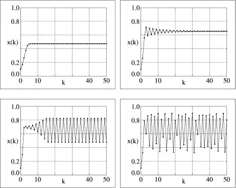
Figure 1.1: Iterations of the logistic map, with parameters (from top left) (i) r = 1.9, (ii) r = 2.9, (iii) r = 3.3, (iv) r = 3.6, all with initial value x₀ =0.1.

(i) For r = 1.9 the population rises rapidly to a steady value of about 0.47 (47% of the carrying capacity), a figure determined by crowding.

(ii) For r = 2.9 the population again stabilises, this time through a sequence of small boom and bust cycles which die out.

(iii) At r = 3.6 the behaviour has become extremely complex, with no apparent pattern or simple repetition. It is in fact chaotic.

(iv) For r = 1.9 the population rises rapidly to a steady value of about 0.47 (47% of the carrying capacity), a figure determined by crowding.

(v) For r = 2.9 the population again stabilises, this time through a sequence of small boom and bust cycles which die out.

(vi) Increasing r to 3.3 changes the behaviour fundamentally. Now the system stabilises on a permanent boom and bust cycle which alternates between good and poor seasons.

(vii) At r = 3.6 the behaviour has become extremely complex, with no apparent pattern or simple repetition. It is in fact chaotic.

Imagine the implications for population control policies if such a simple model can generate such disparate outcomes, depending only on the policy settings!

The above figures were produced by the Iterate (1d) window of Chaos for Java with the Logistic map selected.⁴ Some other interesting values for you to look at before proceeding to the next section include r = 3.5, 3.83 and 4.0.

Financial models

Dynamical models are not just the preserve of the sciences. Two professors of economics, for example, introduced a paper with the words⁵

Imagine a bargaining model … in which each party has been instructed by higher headquarters to respond to each new offer by her opposite number with a counter-offer that is to be calculated from a simple reaction function … If the perfectly deterministic sequence of offers and counter-offers that must emerge from these simple rules were to begin to oscillate wildly and apparently at random, the negotiations could easily break down as each party … came to suspect the other side of duplicity and sabotage. Yet all that may be involved, as we will see, is the phenomenon referred to as chaos …

Needless to say, there is much research on the question of what nonlinear dynamical models and chaos have to say about economics, financial markets,⁶ and investment management. In this respect it is interesting to note that Benoit Mandelbrot, who coined the word fractal, and whose writings had considerable influence in awakening interest in the present subject, first observed the phenomenon of scaling in price changes and income distributions. He stated a pricing principle (hypothesis) as follows (see Mandelbrot [21] chapter 37)

Scaling principle of price change: When X(t) is a price, log X(t) has the property that its increment over an arbitrary time lag d, log X (t + d) − log X (t), has a distribution independent of d, except for a scale factor.

Fractals are treated briefly in chapter 5 of this book; self-similarity of form under changes of scale is one of their hallmarks. An interesting view of how fractals and chaos theory applies to investment theory, including extensive analyses of financial data, may be found in the book of Peters [29].

1.2 Celestial mechanics

The earliest dynamical systems which were the subject of intensive study are concerned with Isaac Newton’s gravitational model of the solar system. A delightful and easily read account of the history of studies into the solar system is given by Ivars Peterson in his book [30]. I shall give only a brief account here.

Newton’s theory gave a satisfactory account of a mass of observations, which had been reduced to three laws by Johannes Kepler. Kepler’s laws are

(i) Planetary orbits are plane ellipses with the sun at one focus.

(ii) A line joining a planet with the sun sweeps out area at a rate constant in time.

(iii) The square of the periods of the orbits are proportional to the cubes of the mean radii.

One sees that the very statement of the laws already takes us a long way toward reducing the data to a dynamical model. They define the important state variables as the positions and velocities of the solar bodies, and they state some relationships, although no theoretical explanation is offered.

The triumph of Newton’s theory is that these laws are explained as the consequence of a simple dynamical model for which he giv...

Table of contents

• Cover
• Half Title
• Title Page
• Copyright Page
• Dedication
• Preface
• Table of Contents
• 1 Introduction
• 2 Orbits of one-dimensional systems
• 3 Bifurcations in one-dimensional systems
• 4 Two-dimensional systems
• 5 Fractals
• 6 Non-linear oscillations
• A Chaos for Java Software
• B Discrete Fourier Transform
• C Variational equations
• D List of Maps and Differential Equations
• Bibliography
• Index