Quantitative Data Analysis in Education

A Critical Introduction Using SPSS

Paul Connolly

• Publisher: Routledge
• Year: 2007
• ISBN:
  9781134191833
• Edition: 1
• Topic: Pedagogía
• Subtopic: Educación general

This book provides a refreshing and user-friendly guide to quantitative data analysis in education for students and researchers. It assumes absolutely no prior knowledge of quantitative methods or statistics. Beginning with the very basics, it provides the reader with the knowledge and skills necessary to be able to undertake routine quantitative data analysis to a level expected of published research.

Rather than focusing on teaching statistics through mathematical formulae, the book places an emphasis on using SPSS to gain a real feel for the data and an intuitive grasp of the main concepts and techniques involved. Drawing extensively upon up-to-date and relevant examples, the reader will be encouraged to think critically about quantitative research and its potential as well as its limitations in relation to education.

Packed with helpful features, this book:

• provides illustrated step-by-step guides showing how to use SPSS, with plenty of exercises to encourage the reader to practice and consolidate their new skills
• makes extensive use of real-life educational datasets derived from national surveys in the US and UK to illustrate key points and to bring the material to life
• has a companion website that contains all of the educational datasets used in the book to download as well as comprehensive answers to exercises and a range of other useful resources that are regularly updated.

The book will therefore appeal not only to undergraduate and postgraduate students but also to more established and seasoned educational researchers and lecturers and professors who have tended to avoid or shy away from quantitative methods.

Chapter 1

Getting started with SPSS

Introduction

The aim of this first chapter is to give you an overview of SPSS and, through this, to show you that handling and analyzing quantitative data need not be difficult. In particular, by the end of this chapter you will:

• understand what a dataset is;

• be able to open an existing dataset with SPSS and also create your own dataset;

• understand the SPSS environment and be able to navigate your way around it;

• have gained some experience of undertaking simple analyses with SPSS;

• be able to save a dataset and also the output of the analyses you have undertaken.

Understanding what a dataset is

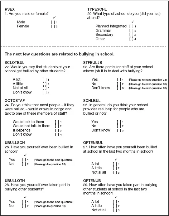
At the heart of quantitative data analysis is the dataset. A dataset is actually just an array of numbers organized into rows and columns. Perhaps the best way to explain it is to start with a real-life example. You will see in Box 1.1 an amended and reduced version of a self-complete questionnaire used as part of the Northern Ireland Young Life and Times Survey 2005. The full questionnaire is much longer than this. All I have done here is to keep two basic questions (what sex the young person is and then what type of school they went to) and then the eight questions in the questionnaire on bullying in school. The layout for the bullying questions is almost exactly as it appears in the original questionnaire.

There are two key things to note from this questionnaire. The first is that each question is given an abbreviated name (i.e. “RSEX,” “TYPESCHL,” “SCLOTBUL” and so on). As will be seen shortly, each question basically equates to a single variable and these abbreviated names are the names used by SPSS for each variable. Many questionnaires of this type do not actually include the variable name like this but simply add them in afterwards. The other thing to note is that there is a number assigned to each of the boxes that the respondent is able to tick. These represent the values that each of the variables can take. Thus for the first question—“Are you male or female?”—the variable name is “RSEX” and this variable only has two values: either “1” or “2,” indicating that the respondent is male or female respectively.

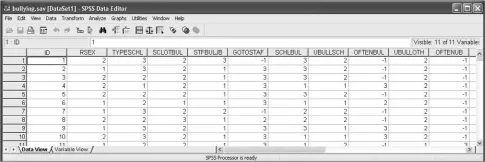
The actual dataset derived from this questionnaire, as it appears in SPSS, is shown in Figure 1.1. You will shortly be asked to open this dataset and explore it. However, for now it is useful just to draw out and highlight two key points from this. First, each row (i.e. horizontal line) represents what is called one case. A case is the term used to refer to the unit of analysis. In this example each case represents one young person who completed the questionnaire. Only the first ten cases are actually visible in Figure 1.1. However, this questionnaire was completed by 819 young people and so there are a total of 819 cases (i.e. 819 rows) in this dataset and they could be viewed simply by scrolling down using the right-hand scroll-bar. The second thing to note is that each column (i.e. vertical line) represents a variable. The name of each variable can be seen at the top of each column and they correspond to and appear in the same order as the variables in the questionnaire itself (Box 1.1). The only additional variable that does not appear in the questionnaire is the first one—“ID”—which is the unique number given to each questionnaire (and thus is a unique number that can be used to identify each case).

Box 1.1 Amended extract from the Northern Ireland
Young Life and Times Survey 2005

All of the numbers that appear in the middle of the screen are basically the values for each of the variables (i.e. the values corresponding to what boxes each respondent ticked). To take the first case as an example (i.e. the first row) then reading across horizontally we can see that their unique ID number is “1,” their sex (“RSEX”) is coded as “2” and the type of school they attend (“TYPESCHL”) is coded as “3” and so on. If we refer back to the original questionnaire we can see that these values mean that this person is therefore female and attends a secondary school. If we continue we can see that the value for the next variable (“SCLOTBUL”) is “2”. Again, referring back to the questionnaire we can see that this means that when asked “Would you say that students at your school get bullied by other students?” this respondent answered “A little.” You can easily continue across the rest of the line to find out how she answered the remaining questions.

The only other thing that needs to be explained are the values of “-1” for the variables “GOTOSTAF” and “OFTENBUL.” These are values added in afterwards by the researcher to indicate that these two questions were skipped by the respondent. To understand this, have a look again at the questionnaire in Box 1.1. For Question 23— “Are there particular staff at your school whose job it is to deal with bullying?”—the respondent is given differing instructions depending on how they answer this question. Thus if they answer “yes” (there is a particular member of staff) then they are asked to go onto the next question (Question 24) which asks how approachable that member of staff is. However, if they had answered “no” or “don’t know” to Question 23, as our first respondent has, then there is no point asking them this next question and so they are instructed to skip it and jump directly to Question 25. In such circumstances, rather than just leaving this variable (“GOTOSTAF”) blank for this respondent a special value, “-1,” is typed in to indicate that this question has been legitimately skipped.

Figure 1.1 The bullying dataset as it appears in SPSS

Before we get you to actually open up and explore this dataset there are three general points to draw from what you have seen so far. The first is that all data need to be translated into numeric form for SPSS to work with (with the exception of descriptive “labels” that we will get onto later). Thus, while the categories that a respondent can choose from for each question are all described in words (e.g. “A lot” or “A little”), we have had to assign them numbers so that they can be entered into the dataset. An important lesson from this is that you should, therefore, think very carefully about how you design your questionnaire to ensure that, as far as possible, the data you gather can be coded in this way. This usually means trying as far as possible to restrict yourself to using closed questions (i.e. questions where there are only a fixed number of response categories to choose from). There will obviously be times when you need to include open-ended questions (i.e. a question that is followed by a space where the respondent writes down their answer in their own words). However, you need to bear in mind that you will have to go back and translate these qualitative answers into codes at some point if you want to analyze them quantitatively. The second key point following on from this is that while numbers have been used for convenience to represent these different categories they may not actually mean anything numerically. Thus while males are coded “1” and females “2” for the variable “RSEX” this has no significance whatsoever. It does not mean, for example, that females are twice as much as males. It could easily have been coded the other way around or using other numbers (i.e. “0” and “1” or whatever). What this means is that we need to be extremely careful in terms of understanding precisely what type of variable we are dealing with and what the values associated with each variable actually represent. This is something we will return to in the next chapter.

The third and final key point to draw from the questionnaire and dataset shown is the usefulness of what is called precoding your questionnaire. Precoding a questionnaire basically means including where possible the variable names and values for each response category on the questionnaire itself. Box 1.1 shows just one of the possible ways that this can be done. The benefit of doing this is in terms of helping to reduce errors that can occur when entering data into SPSS directly from the questionnaire. Imagine, for example, that you have 500 questionnaires of four pages in length and the questions are not precoded and neither are the response categories. In such circumstances it would be very easy to make mistakes typing in the data. If you can precode your questionnaire then whatever box has been ticked you can see immediately which variable it relates to and also what the value is that you need to type in.

Opening an existing dataset in SPSS

Having been introduced to the bullying dataset it is now time to open it up and explore it in a little more detail. First of all you need to download the dataset from the companion website. All the datasets featured in this book are downloadable from the website and you can follow the same routine in each case.

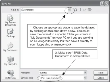
To download and then open the bullying dataset you should begin by going to the companion website and finding the list of datasets. Right click on the link to download the bullying.sav dataset. Select “Save Target As. . .” and this will open the Save As window shown in Figure 1.2. Select an appropriate place to save the dataset using the “Save in:” drop-down menu as shown and also make sure you select “SPSS Data Document” using the “Save as type:” drop-down menu. When you have done this click on the “Save” button. When the download is complete another dialogue box will appear and you should click the “Close” button.

Figure 1.2 Save As window

Open SPSS as you would any other program. For those of you using Windows XP operating system you can do this by clicking on the Start button located at the bottom left of your screen as shown in Figure 1.3. This will bring up the initial SPSS 15.0 for Windows window as shown in Figure 1.4. Make sure that the option “Open an existing data source” is selected and that “More Files. . .” is selected within this and then click “OK.” This, in turn, opens up the Open Data window as shown in Figure 1.5. Make sure you select “SPSS (*.sav)” for “Files of type:” as shown and then use the “Look in:” dropdown menu to navigate around your PC to find the “bullying.sav” dataset where you saved it. Click on the dataset and then click on the “Open” button. You should now have the screen originally shown in Figure 1.1.

Most of the default settings for SPSS are fine and not worth changing. However, one minor change is worthwhile that will help you subsequently when you start exploring and analyzing the data. To make this change select Edit → Options. . . (or SPSS → Preferences. . . if you are using a Mac version). This will open the dialogue box shown in Figure 1.6. To help you find variables quickly and easily for analysis you should change the settings so that SP...