Statistics Tables

For Mathematicians, Engineers, Economists and the Behavioural and Management Sciences

Henry Neave

• Publisher: Routledge
• Year: 2013
• ISBN:
  9781136952173
• Edition: 2
• Topic: Business
• Subtopic: Business General
• Index: Business

For three decades, Henry Neave's Statistics Tables has been the gold standard for all students taking an introductory statistical methods course as part of their wider degree in a host of disciplines including mathematics, economics, business and management, geography and psychology. The period has seen a large increase in the level of mathematics and statistics required to achieve these qualifications and Statistics Tables has helped several generations of students meet their goals.

All the features of the first edition are retained including the full range of best-known standard statistical techniques, as well as some lesser-known methods that can be hard to track down elsewhere. The explanatory introductions to each section have been updated and the second edition benefits from the inclusion of a valuable and comprehensive new section on an approach to simple but powerful investigation of process data. This will help the book continue in its position as the prime statistical reference for all students of mathematics, engineering and the social sciences, and everyone who needs effective methods for analysing data.

Descriptions of the Tables

(References to appropriate books or articles are given for the less familiar topics.)

Section 1: Discrete Probability Distributions

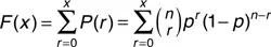
The quantity tabulated in Table 1.1 (pp 20–26) is the cdf (cumulative distribution function) of the binomial distribution:

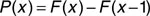
which is the probability of obtaining x or less ‘successes’ in n independent trials of an experiment where at each trial the probability of success is p. Individual probabilities P(x) = Prob (x successes) are easily obtained by using

for x > 0 and P(0) = F(0). The table covers all

and p = 0.01(0.01)0.10(0.05)0.50. For values of

, probabilities may be found by interchanging the roles of ‘success’ and ‘failure’.

Charts 1.2 (pp 27–28) give (a) 95% and (b) 99% confidence intervals for p on the basis of a binomial sample of size n in which there are X successes. If the sample fraction

, locate its value on the bottom horizontal axis, trace up to the two curves labelled with the appropriate value of n, and read off the confidence limits on the left-hand vertical axis; if

use the top horizontal axis and the right-hand vertical axis. For each value of n, the appropriate points have been plotted for all possible values of X/n and these points joined by straight lines to aid legibility. Results for values of n not included may be obtained approximately by interpolation.

The charts may also be used ‘in reverse’ to provide (a) 5% and (b) 1% two-tailed critical regions for the hypothesis test of

against the two-sided

, or equivalently (a)

and (b)

one-tailed critical regions for one-sided tests. (NB ‘One-sided’ and ‘two-sided’ relate to the nature of H₁ and to the relevant tests and statistics; ‘one-tailed’ and ‘two-tailed’ describe the form of critical region.)

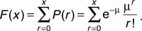
The quantity tabulated in Table 1.3(a) (pp 29–32) is the cdf of the Poisson distribution with mean μ:

Individual probabilities may be found as with Table 1.1. For

the cdf occupies two or more rows of the table, the first row giving F(0) to F(9), the second row F(10) to F(19), etc.

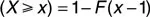
The Poisson probability chart, Chart 1.3(b) (page 33), provides values of Prob

where X has the Poisson distribution with mean μ. The value of μ, ranging from 0.1 to 100, is found on either side of the page and the probabilities are read at the bottom. There is a curve for each of the following values of x: 1(1)25(5)100(10)150. The μ axis has a logarithmic scale and the probability axis a normal probability scale.

Section 2: The Normal Distribution

Table 2.1(a) (pp 34–35) gives values of the standard normal cdf Ф(z) for z = –4.00(0.01)3.00, expressed to four decimal places (4 dp) with proportional parts for the third decimal place of z, and also for z = 3.00(0.01)5.00 to 6 dp. Note that the proportional parts are subtracted if

. Further, by symmetry, i.e. using

, we may also obtain values of

to 4 dp with proportional parts for z = 3.00(0.01)4.00 and to 6 dp for

. If F(x) is the cdf of the normal distribution having mean μ and variance σ², denoted

, then

.

Table 2.1(b) (page 36) gives values of

for a range of values of z from 3.0 to 200.0.

Table 2.2 (page 36) is a brief table of ordinates

of the standard normal pdf (probability density function).

Table 2.3(a) (page 36) provides a selection of useful quantiles (percentage points) of the standard normal distribution, i.e. values of z satisfying

. Six particularly important values are provided to 10 dp. Table 2.3(b) (page 37) is a more comprehensive table of quantiles. Here, for

read q on the right and bottom. For

read q along the left and top and negate the resulting value of z.

Table 2.4(a) (pp 38–39) gives expected values of normal order statistics (normal scores) for sample sizes

, i.e. the values

where

represents a sample of size n from N(0,1) arranged in ascending order. The values are listed in top-down order:

where

, and remaining values may be obtained by symmetry:

. Normal scores are useful in formulating some particularly powerful nonparametric tests (see page 12); the variances of such test statistics usually involve

, and these sums of squares are given in Table 2.4(b) (pp 38–39).

Tables 2.5(a) and (b) (page 40) respectively give moments and quantiles of the distribution of the range R (maximum value – minimum value) of samples from normal distributions for sample sizes up to 20. Denoting the expected (mean) range by E[R] and central moments

of R by r_k, the five columns of Table 2.5(a) respectively give

,

, and

where σ² is the variance of the normal distribution. In particular, the first and second columns give the mean and standard deviation of R in units of σ. Table 2.5(b) gives six quantiles R_{n, q} on either side of the distribution of R, again in units of σ.

Further reading: Table 2.4: Bradley (1968, §6.2); Table 2.5: Lindgren (1976, §7.2.1).

Section 3: Continuous Probability Distributions

Table 3.1 (page 41) gives 13 quantiles t_ν,q of the Student t distribution for degrees of freedom ν covering 1(1)40,45,50(10)100,120,150, ∞. The quantiles are all in the right-hand half of the distributions; values in the left-hand half may be obtained by symmetry:

.

Table 3.2 (pp 42–43) gives 25 quantiles

of the chi-squared (χ²) distribution for degrees of freedom ν covering 1(1)40,45,50(10)100,120, 150,200. Quantiles are provided in both the left-hand and right-hand sides of the distributions since χ² distributions are not symmetric.

Table 3.3 (pp 44–47) gives six right-hand quantiles

of the Snedecor F distribution for the ‘numerator’ degrees of freedom covering ν₁ = 1(1)10,12,15,20,30,50,∞ and the ‘denominator’ degrees of freedom ν₂ = 1(1)25(5)50,60(20)120, ∞. The six quantiles for a particular choice of (ν₁,ν₂) are provided in a block for easy reference, rather than by using a separate page for each value of q. Critical regions for one-sided tests of

against

using the statistic

(where s₁ and s₂ are the adjusted standard deviations of the two samples—see page 91) require critical regions of the form

, so in this case the tables immediately give the required critical values for 100(1 – q)% significance levels. (Interch...

Table of contents

• Cover Page
• Title Page
• Copyright Page
• Preface to the Second Edition
• Table of Contents
• Descriptions of the Tables
• 1 Discrete Probability Distributions
• 2 The Normal Distribution
• 3 Continuous Probability Distributions
• 4 Analysis Of Variance
• 5 Nonparametric Tests
• 6 Correlation
• 7 Random Numbers
• 8 Quality Control and Improvement
• 9 Miscellaneous
• Useful constants
• Sample standard deviations
• Statistics—from classroom to real world
• Asymptotic (large-sample) distributions