Life Cycle Costing for Construction

J.W. Bull

• Publisher: Routledge
• Year: 2003
• ISBN:
  9781135697846
• Edition: 1
• Topic: Architecture
• Subtopic: Architecture Methods & Materials

The construction industry is becoming increasingly aware of the need to adopt a holistic approach to the design, building, and disposal of structures. With 60 per cent of the total construction budget in most developed countries being spent on repair and maintenance, there is an obvious need to design for reliability and durability, with more carefully planned maintenance and repair schedules. One important facet is to look at how costs are distributed and spent during the lifetime of a structure: an approach known as life cycle costing, which has the ultimate aim of minimising total lifetime expenditure. As an example, choosing an inexpensive coating for steelwork may require maintenance every three years, whereas a coating which is more expensive may require repairing only once per decade. It is a question of balance - taking the lifetime costs of the structure into consideration. This new book provides an insight into how whole life costing is affecting our approach to designing, building, maintaining and disposing of structures. The book is written for consulting engineers in the fields of civil and structural engineering, building designers, architects, quantity surveyors, refurbishing specialists, as well as practising civil and structural engineers engaged in planning, design, construction, repair and refurbishment of structures.

1 Introduction to life cycle costing

S.J.DALE

1.1 Introduction

Nowadays we all try to forecast the consequences of our decisions before we proceed although we also know that the odds against a forecast being correct are quite formidable. As the overwhelming majority of people in the construction industry are dealing with someone else’s money it is usual to utilise some form of accepted forecasting method to predict a result.

While the forecast may not be accurate, if suitable parameters are used and all the interested parties concur with the forecasting method, then it is possible that the ultimate psychological goal, that of confidence, which is a prerequisite to investment, may be achieved. If then, by some mischance, the end result is not that intended, at least it can be shown that the decision was based on knowledge at the time.

Most disagreements over finance are a result of a person’s desire not to part with their money. The aim therefore should always be to buy low and sell high. However, more can be paid in the beginning knowing that in the ultimate result the deal will prove to be cheaper or will reap a greater reward. In this event some form of financial analysis of a particular decision becomes necessary. The idea that the economic consequences of a decision can be analysed is logical, and the fact that such an analysis should be recorded for future reference is obviously sensible.

Life cycle costing is a mathematical method used to form or support a decision and is usually employed when deliberating on a selection of options. It is an auditable financial ranking system for mutually exclusive alternatives which can be used to promote the desirable and eliminate the undesirable in a financial environment.

As decision-taking lies at the heart of all our working hours, aids to the taking of decisions are valued and are used to justify our actions. An ability to forecast the consequences of our decisions eliminates uncertainty and forms the basis for ultimate success.

For example, structural engineers know, from the results of laboratory experiments, that a certain size of steel member will support a given load. They can point to the laboratory record as a reason to justify their actions. Usually, the laboratory record will provide several solutions, or sizes of member to support the load. Unsuitable solutions can be eliminated on the basis of special requirement, availability, constructional difficulties or cost. In forming the decision on which steel member to select, the engineer needs to record and justify the final selection. This enables the decision to be audited for effectiveness at some future date.

Usually, the subject of ‘which solution is the cheapest’ has to form part of this decision-making process, and a method of supporting a financial decision needs to be established and recorded to justify such a decision. Life cycle costing can be described as a means of auditing the financial consequences of a decision.

1.2 The problem

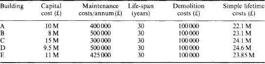
In Table 1.1, five solutions to the specification ‘build an office block’ have been designed and costed. Solution B has obvious financial benefits and therefore will be the selected option. This ‘lowest-cost’ method of decision-making is, without question, the current major method of building option selection and works on the assumption that the cheapest solution is the best financial option.

During the 1930s many building users began to discover that the running costs of the building (i.e. maintenance, energy, management, etc.) began to impact significantly on the occupiers’ budget. It was found that the ‘lowest-cost’ system of selection was not always the cheapest solution over the lifetime of the building. It became obvious that some other method of financial analysis which takes into account the running (or resource) costs of the building must be used to give credence to the decisions when a number of options are under consideration.

Table 1.2 expands the data and changes the decision on the building selection. Over the life of the building option A appears to be the cheapest solution. However, the basis for this decision does not stand up to close inspection. We all know that if maintenance costs are £400000 in the first year of a building’s life they are unlikely to be £400000 in the tenth year of life. This is due to a number of factors such as inflation, replacements, etc. Other factors may also come into play, such as a shortage or glut of raw materials, which would change the base price of a product and could modify the replacement specification (e.g. from timber to aluminium). Similarly, items may require periodic change, over a number of years, resulting in a variable annual maintenance charge. It is clear that a system of financial evaluation that can make allowance for all variables throughout the life of the building and reduce the options to a simple single-figure selection, as in Table 1.1, would make decision-taking a great deal easier.

Table 1.1

Building	Construction cost (£)
A	10 M
B	8 M
C	15 M
D	9.5 M
E	11 M

M = 10³

Table 1.2

M = 10⁶

1.3 The methods

Several options are available. All are well documented and have been in use, certainly since the early 1930s, in many different business sectors. The three most commonly used in the building sector are as follows.

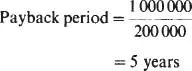
1. Simple payback: defined as the time taken for the return on an investment to repay the investment.

2. Nett present value: defined as the sum of money that needs to be invested today to meet all future financial requirements as they arise throughout the life of the investment.

3. Internal rate of return: defined as the percentage earned on the amount of capital invested in each year of the life of the project after allowing for the repayment of the sum originally invested.

All three methods are accounting systems developed initially for the manufacturing industry to determine the financial worth of an investment. The three methods have been developed to determine if an original investment is worthwhile. For example, the purchase price of (or investment into) a new machine may be £1 million, but extra income earned by the resultant cheaper manufacture, increased production or higher product quality from the machine may be £200000 per annum.

Here the investment generates a known return. In building we generally wish to know if additional money spent on the construction of a building is worth the savings that will be made by a subsequent reduction in running costs. For example, the specification of ceramic tiles in a toilet may be more expensive but the saving in maintenance costs over the alternative painted surface may prove worthwhile.

1.3.1 Simple payback

Simple payback is a simple method of cost appraisal used by many in industry, particularly to evaluate energy-saving schemes. Simple payback can be expressed as:

where P=payback period (years), I=capital sum invested, and R=money returned or saved as a result of the investment.

Thus for our machine example

The decision process now has to decide if five years is an acceptable period for a return on investment capital.

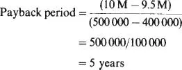
Applying this principle to the options in Table 1.2, it is necessary to adopt a comparator approach to compare solutions A and D. Is the additional investment of £500000 for solution A worth the additional annual saving of £100000 in maintenance costs?

In making a decision to purchase option A rather than option D, it is necessary to assess whether a five-year return on the additional investment is worthwhile.

The use of simple payback is limited by its result. An evaluation of the acceptable payback period is necessary, for which no method or criterion is shown or established. In practice, a maximum period of two or three years is set as a criterion for investment. This is primarily due to the current vogue for a quick return on an investment or ‘short-termism’ but also because the calculation makes no allowance for the following variables:

• Inflation

• Interest (payable or received)

• Cash flow

• Taxation

Reducing the payback period is thought to limit the likely effect of these factors; however, this may not be the case. Considering the effect of taxation alone on the simple ...

Table of contents

• Cover
• Half Title
• Title Page
• Copyright Page
• Preface
• Table of Contents
• 1 Introduction to life cycle costing
• 2 Life cycle costing related to reliability-based and optimum design
• 3 Life cycle costing related to the refurbishment of buildings
• 4 Life cycle costing of highways
• 5 Life cycle costing in the defence industry
• 6 The quality approach to design and life cycle costing in the health services
• 7 How life cycle costing can improve existing costing
• 8 Life cycle cost analysis: a decision aid
• 9 The way ahead for life cycle costing in the construction industry
• Index