Boundary Layer Climates

T. R. Oke

• Publisher: Routledge
• Year: 2002
• ISBN:
  9781134951338
• Edition: 2
• Topic: Physical Sciences
• Subtopic: Geography
• Index: Geography

This modern climatology textbook explains those climates formed near the ground in terms of the cycling of energy and mass through systems.

Part I
Atmospheric systems

1
Energy and mass exchanges

1 ATMOSPHERIC SCALES

The Atmosphere is characterized by phenomena whose space and time scales cover a very wide range. The space scales of these features are determined by their typical size or wavelength, and the time scales by their typical lifetime or period. Figure 1.1 is an attempt to place various atmospheric phenomena (mainly associated with motion) within a grid of their probable space and time limits. The features range from small-scale turbulence (tiny swirling eddies with very short life spans) in the lower left-hand corner, all the way up to jet streams (giant waves of wind encircling the whole Earth) in the upper right-hand corner.

In reality none of these phenomena is discrete but part of a continuum, therefore it is not surprising that attempts to divide atmospheric phenomena into distinct classes have resulted in disagreement with regard to the scale limits. Most classification schemes use the characteristic horizontal distance scale as the sole criterion. A reasonable consensus of these schemes gives the following scales and their limits (see the top of Figure 1.1):

Micro-scale 10^-2 to 10³ m Local scale 10² to 5×10⁴ m Meso-scale 10⁴ to 2×10⁵ m Macro-scale 10⁵ to 10⁸ m

In these terms this book is mainly restricted to atmospheric features whose horizontal extent falls within the micro-and local scale categories. A fuller description of its scope is given by also including characteristic vertical distance, and time scales.

This book is concerned with the interaction between the Atmosphere and the Earth’s surface. The influence of the surface is effectively limited to the lowest 10 km of the Atmosphere in a layer called the troposphere (Figure 1.2). (Note—terms introduced for the first time are italicized and the meaning of those not fully explained in the text is given in Appendix A5.) Over time periods of about one day this influence is restricted to a very much shallower zone known as the planetary or atmospheric boundary layer, hereinafter referred to simply as the boundary layer. This layer is particularly characterized by well developed mixing (turbulence) generated by frictional drag as the Atmosphere moves across the rough and rigid surface of the Earth, and by the ‘bubbling-up’ of air parcels from the heated surface. The boundary layer receives much of its heat and all of its water through this process of turbulence.

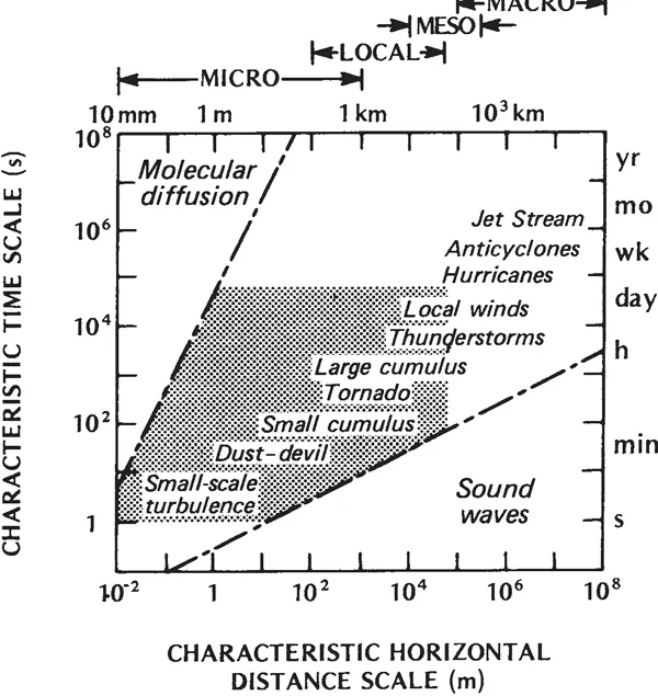
Figure 1.1 Time and space scales of various atmospheric phenomena. The shaded area represents the characteristic domain of boundary layer features (modified after Smagorinsky, 1974).

The height of the boundary layer (i.e. the depth of surface-related influence) is not constant with time, it depends upon the strength of the surface-generated mixing. By day, when the Earth’s surface is heated by the Sun, there is an upward transfer of heat into the cooler Atmosphere. This vigorous thermal mixing (convection) enables the boundary layer depth to extend to about 1 to 2 km. Conversely by night, when the Earth’s surface cools more rapidly than the Atmosphere, there is a downward transfer of heat. This tends to suppress mixing and the boundary layer depth may shrink to less than 100 m. Thus in the simple case we envisage a layer of influence which waxes and wanes in a rhythmic fashion in response to the daily solar cycle.

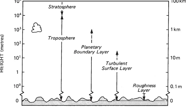
Figure 1.2 The vertical structure of the atmosphere.

Naturally this ideal picture can be considerably disrupted by large-scale weather systems whose wind and cloud patterns are not tied to surface features, or to the daily heating cycle. For our purposes the characteristic horizontal distance scale for the boundary layer can be related to the distance air can travel during a heating or cooling portion of the daily cycle. Since significant thermal differences only develop if the wind speed is light (say less than 5 ms^-1) this places an upper horizontal scale limit of about 50 to 100 km. With strong winds mixing is so effective that small-scale surface differences are obliterated. Then, except for the dynamic interaction between airflow and the terrain, the boundary layer characteristics are dominated by tropospheric controls. In summary the upper scale limits of boundary layer phenomena (and the subject matter of this book) are vertical and horizontal distances of ~1 km and ~50 km respectively, and a time period of ~1 day.

The turbulent surface layer (Figure 1.2) is characterized by intense small-scale turbulence generated by the surface roughness and convection; by day it may extend to a height of about 50 m, but at night when the boundary layer shrinks it may be only a few metres in depth. Despite its variability in the short term (e.g. seconds) the surface layer is horizontally homogeneous when viewed over longer periods (greater than 10 min). Beneath the surface layer are two others that are controlled by surface features, and whose depths are dependent upon the dimensions of the surface roughness elements. The first is the roughness layer which extends above the tops of the elements to at least 1 to 3 times their height or spacing. In this zone the flow is highly irregular being strongly affected by the nature of the individual roughness features (e.g. blades of grass, trees, buildings, etc.). The second is the laminar boundary layer which is in direct contact with the surface(s). It is the non-turbulent layer, at most a few millimetres thick, that adheres to all surfaces and establishes a buffer between the surface and the more freely diffusive environment above. The dimensions of the laminar boundary layer define the lower vertical size scale for this book.

The lower horizontal scale limit is dictated by the dimensions of relevant surface units and since the smallest climates covered are those of insects and leaves, this limit is of the order of 10^-2 to 10^-3 m. It is difficult to set an objective lower cut-off for the time scale. An arbitrary period of approximately 1 s is suggested.

The shaded area in Figure 1.1 gives some notion of the space and time bounds to boundary layer climates as discussed in this book (except that it requires a third co-ordinate to show the vertical space scale). Two aberrations from this format should be noted. First, it should be pointed out that precipitation and violent weather events (such as tornadoes), which might be classed as boundary layer phenomena, have been omitted. The former, although deriving their initial impetus near the surface, owe their internal dynamics to condensation which often occurs at the top or above the boundary layer. The latter are dominated by weather dynamics occurring at much larger scales than outlined above. Second, the boundary layer treated herein includes the uppermost layer of the underlying material (soil, water, snow, etc.) extending to a depth where diurnal exchanges of water and heat become negligible.

2 A SYSTEMS VIEW OF ENERGY AND MASS EXCHANGES AND BALANCES

The classical climatology practised in the first half of the twentieth century was almost entirely concerned with the distribution of the principal climatological parameters (e.g. air temperature and humidity) in time and space. While this information conveys a useful impression of the state of the atmosphere at a location it does little to explain how this came about. Such parameters are really only indirect measures of more fundamental quantities. Air temperature and humidity are really a gauge of the thermal energy and water status of the atmosphere respectively, and these are tied to the fundamental energy and water cycles of the Earth-Atmosphere system. Study of these cycles, involving the processes by which energy and massare transferred, converted and stored, forms the basis of modern physical climatology.

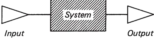
Figure 1.3 Energy flow through a system.

The relationship between energy flow and the climate can be illustrated in the following simple manner. The First Law of Thermodynamics (conservation of energy) states that energy can be neither created nor destroyed, only converted from one form to another. This means that for a simple system such as that in Figure 1.3, two possibilities exist. Firstly:

(1.1)

in this case there is no change in the net energy status of the system through which the energy has passed. It should however be realized that this does not mean that the system has no energy, merely that no change has taken place. Neither does it mean that the Output energy is necessarily in the same form as it was when it entered. Energy of importance to climatology exists in the Earth-Atmosphere system in four different forms (radiant, thermal, kinetic and potential) and is continually being transformed from one to another. Hence, for example, the Input energy might be entirely radiant but the Output might be a mixture of all four forms. Equally the Input and Output modes of energy transport may be very different. The exchange of energy within the Earth-Atmosphere system is possible in three modes (conduction, convection and radiation (see Section 3 for explanation)).

The second possibility in Figure 1.3 is:

For most natural systems the equality, Input=Output, is only valid if values are integrated over a long period of time (e.g. a year). Over shorter periods the energy bala...

Table of contents

• COVER PAGE
• TITLE PAGE
• COPYRIGHT PAGE
• ACKNOWLEDGEMENTS
• PREFACE TO FIRST EDITION
• PREFACE TO SECOND EDITION
• SYMBOLS
• PART I: ATMOSPHERIC SYSTEMS
• PART II: NATURAL ATMOSPHERIC ENVIRONMENTS
• PART III: MAN-MODIFIED ATMOSPHERIC ENVIRONMENTS
• APPENDIX A1: RADIATION GEOMETRY
• APPENDIX A2: EVALUATION OF ENERGY AND MASS FLUXES IN THE SURFACE BOUNDARY LAYER
• APPENDIX A3: TEMPERATURE-DEPENDENT PROPERTIES
• APPENDIX A4: UNITS, CONVERSIONS AND CONSTANTS
• APPENDIX A5: GLOSSARY OF TERMS†
• REFERENCES
• SUPPLEMENTARY READING