Geographies of Labour Market Inequality

Ron Martin, Philip S. Morrison

• Publisher: Routledge
• Year: 2003
• ISBN:
  9781134421572
• Edition: 1
• Topic: Architecture
• Subtopic: Urban Planning & Landscaping

In recent years, the local dimensions of the labour market have attracted increasing attention from academic analysts and public policy-makers alike. There is growing realization that there is no such thing as the national labour market, instead a mosaic of local and regional markets that differ in nature, performance and regulation. Geographies of Labour Market Inequality is concerned with these multiple geographies of employment, unemployment, work and incomes, and their implications for public policy.

Part I

The production of local labour market inequalities

2 Labour market risk and the regions: evidence from gross labour flows

Philip S. Morrison and Olga Berezovsky

Introduction

Risk society, as Ulrich Beck uses the term, ‘describes a phase of development of modern society in which the social, political, ecological and individual risks created by the momentum of innovation increasingly eludes the control and protective institutions of industrial society’ (Beck, 1999: 72). Although Beck is concerned with ‘society at large’, it is clear that some of its members are exposed to substantially higher risks than others.¹ Our particular interest here is in aspects of risk in the labour market, and especially in less secure regional labour markets. In this chapter we show how the concept of risk not only highlights the geographic variability of the labour market but alters search behaviour in ways that feedback into indicators we use to judge the economic health of regions.

Gross flows refer to flows of the working age population between three mutually exclusive labour market states: employment, unemployment, and outside the labour force. Measured over months or quarters, these flows indicate the proportion of people entering and leaving the labour market as well as those moving from employment and unemployment within it. The nine possible flows that interconnect the three states collectively depict the dynamics. The study of labour market flows can be traced back at least as far as the 1960s. Holt and David (1966), for example, were concerned with the way searching individuals matched job vacancies and how this influenced the behaviour of key magnitudes like unemployment. Most of the early empirical work focused on the behaviour of the working age population as they moved between labour market states (see for example Perry, 1972; Marston, 1976; Clark and Summers, 1979; Foster, 1981; Foster and Gregory, 1984; Blanchard and Diamond, 1990, 1992; Burgess, 1994; Davis and Haltiwanter, 1999). More recently attention has shifted to the efficiency of the vacancy–worker matching process (e.g. Burda and Wyplosz, 1994; Barkume and Horvath, 1995 and Beeson Royalty, 1998).

Despite the insights gained through the study of gross flows at the aggregate level there have been very few applications at sub-national scales (see Schettkat, 1996a; Lazar, 1977; Armstrong and Taylor, 1983, 1985; Martin, 1984; Green, 1986; Jones and Martin, 1986; Gorter et al., 1990; Jones, D.R., 1992; Jones, S.R.G., 1993, 1998a; Bennett and Pinto, 1994; Martin and Sunley, 1999). Nevertheless one can trace some of the basic ideas back much earlier, see Singer (1939). The same is true for the work on matching functions although recently several applications using regional data have begun to appear (e.g. Ritter, 1993; Gorter and van Ours, 1994; Broersma, 1997; Mortensen, 1994). When regional gross flows have been analysed it has been primarily to measure the relative importance of gross flows into and out of unemployment. Although collectively results of this regional research have been modest they have at least established that the dynamics underlying the unemployment rate do differ substantially from one region to another.² By contrast, relatively little attention has been paid to the regional dynamics of the other main states, to the gross flows into and out of employment and the labour force as a whole.

In this paper we argue that the dynamics which underlie employment levels are of particular interest in regional and local labour market contexts because of the local multiplier effects of earned income. Losses which fall unevenly on people grouped by age, gender, or occupation alone are geographically diffused, but when they are grouped by place the adverse effects of employment loss generate negative externalities and compound themselves locally. For example, if the number employed falls severely in a locality then local spending falls, trade declines, net out-migration increases and the declining labour pool can lead to the net out-migration of further potential employers. When it comes to understanding the standard of living in a region and regional inequality it is the risk of leaving employment rather than simply the likelihood of becoming unemployed that is important.

One of the reasons for the limited attention paid to gross flows at the regional level is the lack of appropriate data. The release of full gross flows data at the regional level by Statistics New Zealand for this study opens up opportunities to explore the dynamics that lie behind all three key rates; the unemployment rate, the employment rate and the labour force participation rate. It is the movement in and out of employment which is of particular concern in this chapter.

The use of panel data to study labour markets, although well established internationally, has been realised only lately in New Zealand. Even though a feasibility study was undertaken in 1976 and government approval was obtained in 1979, the Household Labour Force Survey (HLFS) did not start producing data until the last quarter of 1985. Gross labour flow analysis was not applied until the 1990s when sufficient number of years of the household labour force survey had elapsed to provide adequate information (see Grimmond, 1993a; Silverstone and Gorbey, 1995; Gardiner, 1995; Herzog, 1996; Irvine, 1995; Wood, 1998).

As of the late 1990s, the data published from the HLFS was based on a questionnaire applied quarterly to a stratified sample of over 15,000 private dwellings throughout New Zealand.³ Information is obtained on each resident in the dwelling yielding about 30,000 individual respondents each quarter.

Households remain in the sample for two years, one-eighth of sample households being rotated out of the survey each quarter and replaced by a sample of new households. In their first quarter households are interviewed in person regarding their participation in the labour market and then again by telephone over the successive quarters. Measures of change in the numbers employed, unemployed and those outside the labour force are based on the matched households only, that is the seven-eighths of the survey that remain in the sample from quarter to quarter.⁴

The remainder of the chapter is organised as follows. We begin with an overview of labour market dynamics in Auckland, the most heavily population region of New Zealand. This allows us to introduce the data sources, concepts and magnitudes involved in gross flows analysis. The subsequent section then outlines the model used to estimate the risk of leaving employment and the subsequent section presents the results. We then discuss a number of issues arising from the use of gross flows in general and at a regional level, and end with some conclusions and implications.

Labour market dynamics

Geographers, regional scientists and those economists who venture into subnational issues have tended to describe the labour market conditions of regions by using rates, particularly the unemployment rate (e.g. Vedder and Gallaway, 1996; Martin, 1997; also see Gleave and Palmer, 1980), and the labour force participation rate (e.g. Gordon, 1970, Elhorst, 1996, 1998, Greenhalgh, 1977, Molho, 1983 and Gallaway et al. 1991). These rates are based on stocks constructed from the standard classification of the working age population into the employed (E), unemployed (U) and those not-in-the-labour force (N). The unemployment rate is calculated as u = U/(U + E), and the labour force participation rate as l = (E + U)/(E + U + N).

One of the aims of this chapter is to reinterpret the conventional U and N categories explicitly in labour search terms and to explore the way in which the different forms of search which they represent are used under different regional labour market conditions. The job search questions typically asked in household labour force surveys allow us to empirically identify individuals according to the degree of search activity. Following international practice, New Zealand defines the ‘unemployed’ as those in the working-age population who are without a paid job, available for work, and actively seeking work in the four weeks ending with the reference week (or are starting a new job within four weeks). For reasons expressed by Clark and Summers (1979) and others (e.g. Gonul, 1992) about the narrowness of this definition, we have extended this conventional notion of unemployment to include those who were without employment (during the reference week) and available (but not actively seeking work) as well as those actively seeking (but not available for work), plus those who seek work through newspapers only. The result is a new wider category of unemployed we call the jobless. By using the jobless (J) measure we not only reduce much of the ambiguity surrounding the narrow official definition of the unemployed but we nearly double the number of ‘unemployed’, thus reducing the sampling error typically associated with this gross flows category.

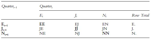
Table 2.1 Gross flow addresses

Our analysis of gross flows in the New Zealand regional context will therefore be based on flows between three categories: the employed E, the jobless J and those outside the labour force N. In order to illustrate the typical pattern of labour market flows that can be generated in this way we take the reader through an analysis of the quarter-by-quarter flows of male workers in Auckland, the largest of the New Zealand regions. As well as offering a convenient illustration of the gross flows method, the Auckland case also serves as the base against which to compare the experience of other New Zealand regions.

Illustration of gross flows

Table 2.1 labels each of the flows between the time periods Q_t-1 and Q_t in the standard gross flows matrix. So for example, EJ refers to the flow of people from the state of employment in the previous quarter, t–1, to the state of joblessness (J) in the next, t. The cell EN denote flows over the same period from employment to not-in-the-labour force, and the cell EE counts the number who remained in employment from one quarter to the next, and so on for the remaining six cells in the matrix. The three entries in main diagonal of the matrix {EE, JJ and NN} refer to individuals who have not changed their status from quarter to quarter. The six off-diagonal cells count those who have made a transitions {EJ, EN, JN, JE, NE and NJ}. The rightmost column E, J and N. refer to the number in each category at the beginning of the period; they are the sums of the row entries, e.g. E. = EE + EJ + EN.

The gross flows of male workers in the Auckland region is described in Table 2.2 for the 3/91 to 4/91 period. The table shows first how the 289.8 thousand men of working age surveyed in the third quarter of 1991 were distributed over the three states: 143.1 or 49.5 per cent were employed, 27.5 thousand or 9.5 per cent were unemployed and the remainder, 118.9 thousand or 41 per cent lay outside the labour force.⁵ Summing the off-diagonal entries reveals that an estimated total of 40.1 thousand men or 14 per cent of the region’s working age population changed their labour market state within the space of only three months.⁶

Table 2.2 The gross flows matrix. Males in the Auckland region between quarters 3 and 4, 1991 (in thousands)

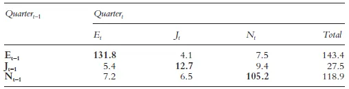
Source: Statistics New Zealand, Special tabulation from the Household Labour Force Survey.Rounded to the nearest 100.

Table 2.3Transition probabilities of males in the Auckland region, quarter 3–4,1991

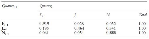
Source: Statistics New Zealand. Special tabulation from the Household Labour Force Survey.

The sheer volume of ‘churning’ (or ‘turnover’) within this regional labour market is impressive, but it is typical of both national and regional markets in general. In terms of learning how the regional labour market functions, however, it is not the absolute number moving that is most useful but the normalised values, that is the probability that an individual in any given state will in fact change state within the time period. For example, the probability that an individual who is employed in t_-1(E_-t-1) will become jobless (J) in t is EJ/E which, from Table 2.2, is 0.028 = 4.1/143.4 or about three out of every one hundred employed.

It is apparent from the full set of transition probabilities in Table 2.3 that as a group the employed in Auckland are relatively stable with over 9 out of 10 male workers remaining employed from one quarter to the next. The next most stable group are those outside the labour force, 8.8 out of 10 staying outside for the duration of the quarter. By contrast, the unemployed are quite unstable–even in this application where we have doubled the size of this category by making it refer to the jobless. Less than half of those who were jobless in one quarter were recorded as such in the following quarter.

We also learn from Table 2.3 that only about 20 per cent of those leaving joblessness actually move into employment (JE), that just under half remain jobless (JJ), and that over one-third leave the labour force altogether (JN). This high propensity to leave (and re-enter) the labour force is one of the big revelations from the extensive empirical literature on gross flows. The more general point is that few of the features that emerge from Table 2.3 are unique to Auckland or New Zealand but are characteristic of gross flows matrices over a range of countries.⁷

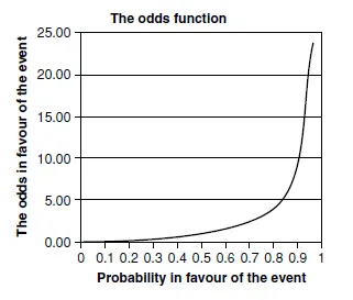
Figure 2.1 Transforming probabilities into odds.

Space does not permit us to analyse all the flows in such a matrix and for the purposes of this chapter we will focus primarily on the first row–what happens to the employed. We will focus not only on the likelihood that men will l...

Table of contents

• Front Cover
• Geographies of Labour Market Inequality
• Title Page
• Copyright
• Contents
• List of contributors
• Preface
• Introduction
• PART I The production of local labour market inequalities
• PART II Interventions and policies
• Postscript
• Index