Financial Modelling and Asset Valuation with Excel

Morten Helbæk, Ragnar Løvaas, Jon Olav Mjølhus

• Publisher: Routledge
• Year: 2013
• ISBN:
  9781134620272
• Edition: 1
• Topic: Business
• Subtopic: Business General
• Index: Business

Finance is Excel! This book takes you straight into the fascinating world of Excel, the powerful tool for number crunching. In a clear cut language it amalgamates financial theory with Excel providing you with the skills you need to build financial models for private or professional use. A comprehensive knowledge of modeling in Excel is becoming increasingly important in a competitive labour market.

The chapters in part one start with the most basic Excel topics such as cell addresses, workbooks, basic formulas, etc. These chapters get more advanced through part one, and takes you in the end to topics such as array formulas, data tables, pivot tables, etc. The other parts of the book discusses a variety of subjects such as net present value, internal rate of return, risk, portfolio theory, CAPM, VaR, project valuation, asset valuation, firm valuation, loan, leasing, stocks, bonds, options, simulation, sensitivity analysis, etc.

Part I

Excel

Excel, which is a part of Microsoft Office, is a spreadsheet program. This computer program has been developed over many years, and is today the market leader of spreadsheet programs.

This book uses Excel 2010, which includes some changes compared to Excel 2007. The 2010 version is available in a 64-bit version which offers increased capacity and makes it easier to work with large and complex spreadsheets. The ribbon in Excel 2010 includes some new tools, the most important being the File button which opens the backstage view.

Part I is an introduction to Excel with demonstrations spanning from basic methods to more advanced applications. Tips showing how to work more effectively and how to build functional models are also included. Those who want to learn even more may consult more comprehensive textbooks on Excel or search on the Internet.

Excel consists of the modules spreadsheet, charts, VBA (Visual Basic for Applications) and several library functions. This part discusses spreadsheets, charts and a few library functions. VBA will be discussed in Part V.

1 Getting started

1.1 Workbooks and spreadsheets

An Excel file is called a workbook and consists of one or several spreadsheets. A spreadsheet is built up by many cells that may contain text, numbers or formulas that refer to other cells. Each cell has an address defined by a column number (from 1 to 1 048 561) and a row number (from A to XFD).

The nice thing about Excel is that you can perform operations on the numbers or the text written in the cells. You can do calculations in a budget, complex mathematical calculations, operations on a text, etc.

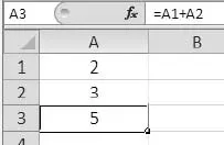
In figure 1.1 the numbers 2 and 3 are written in the cells A1 and A2 respectively. A formula in Excel always starts with a “=”. In cell A3 we have written the formula “=A1+A2” so that the content in the cell becomes 5. When writing the formula we do not have to write “A1”. It is much easier to click on the cell A1 to get the cell address written in the formula. Formulas will be discussed further in chapter 2.

Figure 1.1 A formula in Excel.

The screen

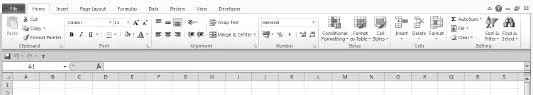
When you start Excel, the first spreadsheet in a workbook opens with menus and options shown on a ribbon (see figure 1.2). The ribbon is divided in several tabs (File, Home, Insert, etc.) where each tab contains a number of groups. Figure 1.2 shows the different groups (Clipboard, Font, etc.) under the tab Home. Each group offers several choices. The group Font, for instance, offers different choices for formatting. To the right and at the bottom of this group, we find an arrow. If we click on it, a dialogue box with more choices appears on the screen.

Figure 1.2 The ribbon in Excel 2010.

The tab File at the left of the ribbon is green and is something new in Excel 2010. When we click this tab, we enter a so-called backstage view where we can save, print and administer our files.

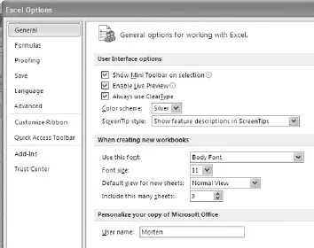
When we click Options in the backstage view, the Excel Options dialogue box appears as shown in figure 1.3. Here we can change the contents of the ribbon, choose what we want to appear on the Quick Access toolbar, etc. We will return to this toolbox and to the ribbon later in this and in other chapters.

Figure 1.3 The Excel Options dialogue box.

The Quick Access toolbar is shown under the ribbon in figure 1.2. It’s a good idea to include the most commonly used commands in this toolbar. We can do that from the dialogue box in figure 1.3 or by clicking the arrow symbol on the Quick Access toolbar.

Below the Quick Access toolbar we find the formula bar which shows the content of the active cell. At the left on this line, we find a window with the address of the active cell.

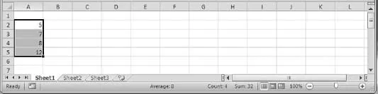
Figure 1.4 illustrates the lower part of a spreadsheet. The three spreadsheet tabs (Sheet1, etc.) represents three different spreadsheets. The line at the bottom is called the status bar and offers different choices. We may for instance increase or decrease the size of the cells.

In figure 1.4 the cells A2:A5 contains some values. When these cells are marked, the average, the number of values, and the sum of the values appears on the status bar. We can change the status bar by right-clicking on it and choosing the desired information from the menu that appears.

Figure 1.4 Spreadsheet tabs and status bar.

Organizing your workbooks

Every time you open Excel, a new workbook with empty spreadsheets appears on the screen. Excel also offers several templates, which are workbooks designed for different purposes. To enter one of these templates, click the File tab and then New. It is also possible to create your own templates in Excel.

The height of rows and the width of columns can easily be changed by clicking and pulling the lines between two row or column headings. If you right-click on a series of marked row or column headings, a menu appears where you can hide the row or column, choose a desired height or width, etc.

If you want to look at one part of a spreadsheet and move (vertically or horizontally) on another part, mark a row or a column by clicking the heading, click the tab View and choose Freeze Panes in the group Window. Then the cells over the marked row (or to the left of the marked column) will be frozen while you scroll through the rest of the spreadsheet. If you start this procedure standing in a single cell, the cells over and to the left of the cell will freeze.

If you want to work with various workbooks at the same time, open the desired workbooks, click the tab View, and choose Arrange All in the group Window. Then you will get the dialogue box in figure 1.5, where, among other things, you can choose to place the workbooks side by side.

You can also open multiple copies of the same spreadsheet. To do this, first choose the tab View and then New Window under the group Window. Then you can sort the copies of the spreadsheet as described above.

If you need to make drastic changes to a spreadsheet, right-click the spreadsheet tab (at the bottom of the screen). Then you will get a menu where you can delete the spreadsheet, add new spreadsheets, move the spreadsheet to a different document, etc. You can also change the order of the spreadsheets in a workbook by clicking and pulling the spreadsheet tabs. If you hold down the Ctrl-button while clicking and dragging a sheet tab, a copy is made of the spreadsheet.

If you want to delete more than one spreadsheet, hold down the Ctrl-key and click the spreadsheets’ tabs of current in...

Table of contents

• Cover Page
• Half Title page
• Title Page
• Copyright Page
• Contents
• List of figures
• List of tables
• Part I Excel
• Part II Basic finance
• Part III Valuation
• Part IV Simulations
• Part V VBA
• Index