Income Distribution and Environmental Sustainability

A Sraffian Approach

Robin Hahnel

• Publisher: Routledge
• Year: 2016
• Print ISBN:
  9781138229129
• eBook ISBN:
  9781315390222
• Topic: Business
• Subtopic: Business General
• Index: Business

Any economics that does not deal forthrightly with economic inequality is no longer suitable for the twenty-first century. Similarly, any economics which does not provide a coherent way to integrate environmental sustainability into economic analysis will fail to command allegiance in the century ahead. This book demonstrates how the Sraffian framework provides important advantages in both areas.

Divided into three chapters, Income Distribution and Environmental Sustainability provides a rigorous exposition of Sraffian theory emphasizing what it means for the economy to be productive, extends Sraffian theory to address environmental sustainability, and adds a normative theory of income distribution to Sraffa's positive theory. In Chapter 1, a rigorous version of the basic Sraffa model is presented which focuses on what it means for the economy to be capable of producing a physical surplus, explains the origin of profits, and shows how to measure changes in overall labor productivity resulting from any technical change. In Chapter 2, the basic model is extended to incorporate primary inputs from the natural environment, rigorously measure changes in environmental throughput efficiency, and establish sufficient conditions for environmental sustainability. In Chapter 3, an explicit "normative" theory of economic justice is elaborated which is a natural extension of Sraffa's "positive" theory of income determination and consistent with modern egalitarian literature on distributive justice.

This book is of interest to academics and students who study political economy, economic theory, and philosophy, as well as those interested in the work of Piero Sraffa.

1 Sraffa after Frobenius–Perron

1.0 Introduction to Chapter 1

Chapter 1 develops a rigorous version of basic Sraffian theory as a sequence of theorems. While much of Chapter 1 covers familiar ground, the emphasis on what it means for the economy to be productive and how we are to understand the origin of profits differs from many presentations. The critique of what we might call Adam Smith’s second invisible hand, namely that profit maximizing capitalists can be relied on to choose efficient technologies, and theorem 18, which clarifies the relationship between dominant eigenvalues of socio-technology matrices, profitability, and productivity, break new ground.

Theorems which are important to the economic argument are proved in the main body. However, for the convenience of readers seeking a self-contained text, proofs of some theorems due to Frobenius and Perron, as well as demonstration of the equivalence of different definitions of what it means for an economy to be productive, are provided in Appendix A.

1.1 Mathematical notation, definitions, and theorems

a. Mathematical notation

A, an (n, n) matrix of direct inputs of produced goods, where a(i j) is the number of units of good i needed to produce one unit of gross output of good j.

a(j), the jth column of A, a (n, 1) column vector representing the direct inputs of produced goods needed to produce one unit of gross output of good j.

a(i), the ith row of A, a (1, n) row vector representing the amounts of good i needed as direct inputs to produce one unit of gross output of each and every good.

(I − A)⁻¹, an (n, n) matrix of direct and indirect inputs, where A(i j) is the amount of good i needed directly and indirectly to produce one unit of good j.

L, a (1, n) row vector of direct labor inputs, where l(j) is the number of hours of labor required, along with all the produced inputs needed, to produce one gross unit of good j.

b, an (n, 1) column vector where b(i) is the consumption of good i per hour of labor worked. In other words, b is the real, hourly wage consumption vector.

A* = [A + bL], an (n, n) matrix called the “augmented” or “socio-technology” input matrix. a*(i j) = [a(i j) + b(i)l(j)] represents the sum of the amount of input i required directly as material input to produce one gross unit of good j and indirectly in the form of consumption of good i by workers producing one unit of good j.

a*(j), is the jth column of A*, an (n, 1) column vector representing the inputs needed to produce one unit of gross output of good j, both directly as material inputs and indirectly in the form of consumption by workers producing one unit of j.

p, a (1, n) row vector of good prices, where p(j) is the price of good j.

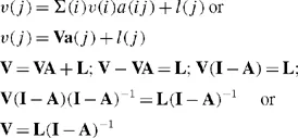
V, a (1, n) row vector of “labor values,” where v(j) is the number of hours of labor it takes directly to produce one unit of good j, l(j), plus the number of hours it took to produce all the produced inputs, a(j), needed to produce a unit of j. In other words, v(j) is the total number of hours it took to make a unit of good j, both directly and indirectly.

Note: the “value” of good j, v(j), and the vector of labor “values” for the economy, V, can be calculated as follows:

x, an (n, 1) column vector of gross outputs produced, where x(i) is the number of units of gross output of good i.

f, an (n, 1) column vector of net, or final outputs, where f(i) is the number of units of net output of good i produced. Note: f = x − Ax.

r(j), a pure number, the rate of profit in sector j.

r, a pure number, the uniform rate of profit in the economy.

w, a scalar, the hourly wage rate.

Note: if we say A > B, we mean that each and every element of matrix A is greater than its corresponding element in matrix B. If we say A≥Y we mean that no element in A is less than its corresponding element in Y, and at least one element in A is greater than its corresponding element in Y.

b. Non-negative, indecomposable matrices

A square matrix, A (n, n), is defined as non-negative and indecomposable if:

(i) a(i j) ≥ 0 all i, j (non-negative); and

(ii) for each (i, j) there exists a set of indices such that a(ik1)a(k1k2)… a(kmj) > 0 (indecomposable).

c. Frobenius–Perron theorems

Theorems 1 and 3 are originally due to Frobenius and Perron. Theorem 1 is often called the Frobenius–Perron theorem, while theorems 1 and 3 taken together are often referred to as the full Frobenius–Perron theorem. The remainder of the theorems on non-negative, indecomposable, square matrices listed below are derivatives of the work of Frobenius and Perron, and will be used at different points in developing the surplus approach. Proofs of all theorems are in Appendix A.

(T1) Theorem 1. If A is non-negative and indecomposable, there exists an α, x*, and p* such that:

(i) Ax* = α x* with α > 0 and x* > 0;

(ii) p*A = α p* with p* > 0;

(iii) α , the dominant eigenvalue of A, dom(A), is unique, and x* and p* are unique up to a multiplicative constant.

(T2) Theorem 2. For k > 0:

(i) if for some z ≥ 0, Az ≥ kz, then α = dom(A) > k;

(ii) if for some z ≥ 0, Az ≤ kz, then α = dom(A) < k;

(iii) if for some z ≥ 0, zA...

Table of contents

• Cover
• Half Title
• Title Page
• Copyright Page
• Table of Contents
• List of figures
• Acknowledgments
• Introduction
• 1 Sraffa after Frobenius–Perron
• Appendix A: Proofs of mathematical theorems
• 2 Environmental sustainability in a Sraffa model
• 3 Producers and parasites
• Appendix B: Reward for effort and modern theories of distributive justice
• Conclusion
• References
• Index