The Economic Theory of Fiscal Policy

Bent Hansen

• Publisher: Routledge
• Year: 2014
• ISBN:
  9781317833505
• Edition: 1
• Topic: Business
• Subtopic: Business General
• Index: Business

The book explores whether fiscal policies can secure full employment without inflation, one of the key questions in economics after Keynes. Part 1, General Theory of Public Finance and Fiscal Policy, discusses Ends and Means in economic policy. The results of this ends-means analysis are applied to fiscal policy. Part 2, Microeconomics, deals with the impact of fiscal measures on the behaviour of the individual household, firm and other organization, concentrating on the effects on consumption and saving. Part 3, Macroeconomics, considers how the problem of keeping the price-level constant and the labour market in equilibrium at full employment may be solved by means of fiscal and monetary measures. Problems connected with the volume of investments and the balance of payments are considered simultaneously.

PART I

GENERAL THEORY OF FISCAL POLICY

Problems and Methods

CHAPTER I

Ends and Means in Economic Policy

1. ENDS AND MEANS IN ECONOMIC MODELS

THE question of how the stabilization of prices can be brought about at full employment—whatever meaning is given to these terms—is a typical example of the more general question of how certain ends can be realized by using certain economic means. Thus there is good reason for discussing the general relationship between ends and means in economic policy. It must be said at once that the end-means problems which will be investigated here are not the deep or pseudo-philosophical problems that are often discussed under this heading. It is a purely technical question of the relationship between ends and means in economic models that is our concern here. The discussion will take place on a rather formal plane, but it will be illustrated to some extent by the ends of full employment and a stable value of money, and certain means for attaining these ends—monetary and fiscal policy.

2. AN ABSTRACT MODEL

Let us consider a completely abstract, ‘exact’ model consisting of n equations, φ_i = 0, containing m parameters, a_j, and determining the value of n unknowns, x_i; thus:

The equations are supposed to be independent and consistent; the system has only one solution in the x_iS. With given values of the parameters the value of x_i is determined. For example, let the m parameter values be a_j⁰; the value of the n unknown variables are then, x_i⁰.

Model (I: 1) is supposed to contain all the a priori knowledge, that we believe to be correct about the economy in which we are interested. We presuppose that our theory can be expressed in terms of such a system of equations. The x_iS are the variables we wish to explain: the endogenous variables; the a_jS are determined outside the system. The endogenous variables may be dated or undated, i.e. the system may be dynamic or static. The discussion throughout Part I deals with both static and dynamic models.¹

In order to illustrate this more closely we shall have to consider a simple dynamic model with the equations for the period t (x_{1, t} denotes the variable x₁ in time t, a_{j, t} denotes the parameter a_j in time t, etc.):

As can be seen we have dated the parameters. Even if these are determined outside the system, there is no reason to presume that a certain parameter, e.g. a₁, should have the same value at all points of time. Especially as the State has at its disposal some of the parameters (cf. section 3) it seems natural that the possibility must be recognized that the parameter values change from period to period.

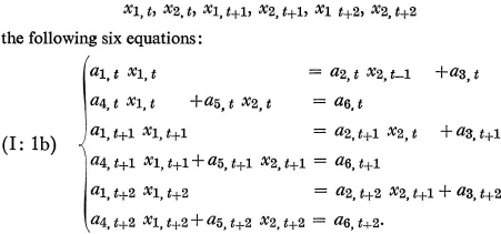
If we are now interested in the happenings of the first three periods—the horizon comprises those periods—we have for the determination of the six endogenous variables

When the dynamic system has been explicitly written down in this way for all the periods within the horizon the system can be treated formally just like any other system of simultaneous equations.² The fact that the variables x_{1, t}, x_{1, t+1} etc. are separated in time is without relevance as far as the purely formal method of analysis is concerned. Instead of taking x_{1, t} and x_{1, t+1} as different values of the same variable at two different points of time, we quite simply interpret them as two different endogenous variables; the dating will then only be a method of distinguishing the variables and in our example we have six equations with six unknowns. The formal treatment of static and dynamic systems will in this way be quite similar; so, for example, the dynamic system above can be differentiated in the usual way in order to get an expression for the effect on a certain variable some time in the future of a current parameter change, that is an expression like ∂x_{1, t+2}/∂a_{2, t} etc. Thus, when we use derivatives in the following chapters in order to denote the effects of parameter changes, the differential in the numerator can very well be given a dating separate from the dating of the differential of the denominator. Then the analysis gets the character of a ‘comparative dynamics’. Another thing, of course, is that dynamic models written down in this explicit way will have certain characteristics differing from those of ordinary static models, which also consist of such systems of equations. In a dynamic model derivatives having numerator differentials of an earlier dating than the denominator differentials will always be zero.

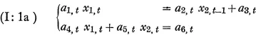
In this context the concept of ‘exogenous’ variables or ‘exogenous’ factors can be mentioned. It follows from the above that there is no room in the system (I: 1) for ‘exogenous’ factors. All symbols were classified as either endogenous variables or parameters. As we have chosen to write down all the equations as one system, we actually have no greater use for the concept of exogenous factors; when and if such appear in the system they could be included among the parameters. If, for instance, we consider the system (I: 1a) x_{2, t−1} is exogenous in the ordinary meaning; if each equation is considered on its own, x_{1, t} is furthermore an exogenous variable in the second equation. In the same way likewise with system (I: 1b). If we consider this as a whole, x_{2, t−1} occurs as the only exogenous factor and it could well be included among the parameters. The reason that we choose this perhaps somewhat unusual method is of course that we wish to deal with static and dynamic, interdependent and non-interdependent systems together.

3. DEFINITIONS OF THE CONCEPTS OF ENDS AND MEANS

With the model (I: 1) as a background we shall now define the concepts of ‘end’ and ‘means’. By an economic ‘end’ is meant a restriction on the endogenous variables, e.g. that a certain variable, say x_k, will take on a definite value, say

_k. Every restriction on the endogenous variables, which is added to the system (I: 1) is an additional end. For example, if it is wished to give three different endogenous variables certain definite values, this is reckoned as three ends. By ‘means’ on the other hand, we quite simply mean the parameters of the model. Each parameter is a means; the extent of a change in a parameter will then be an indication of the extent to which the means is used.

Where the definition of an ‘end’ is concerned there is hardly any difficulty, at least, if by ‘end’ is meant economic end; which variables that should be counted among the endogenous variables, are decided by what are conventionally considered as ‘economic’ variables. The identification between ‘means’ and parameters, on the other hand, is perhaps more difficult to accept. For that reason the meaning of the concept of a parameter will be explained further.

A parameter symbolizes a factor which influences the endogenous variables, without being affected itself by them. So far the distinction between endogenous variables and parameters is clear. It is of no real importance, however, how one differentiates between parameters and the function forms. Parameters can always be written explicitly or included in the functional symbols, which would then have to be changed. All parameters are considered to be ‘autonomous’ in the sense that one can always change a certain parameter without thereby affecting the other parameters (by reason of relationships that exist between the parameters outside the model).

Having defined the concept of the parameter in this way, it is convenient to classify parameters according to the following principles. We distinguish between ‘controllable’ and ‘uncontrollable’ parameters and between ‘permitted’ and ‘non-permitted’ parameters. The dividing line between the controllable and uncontrollable parameters is based on the fact that certain parameters, the uncontrollable, may be considered to be given by ‘nature’, while the remainder can be determined by those who determine economic policy.³ The fact that a parameter is controllable does not however imply that the policymaker can ascribe any value he chooses to it. His control over it can be limited to a greater or lesser extent. The dividing line between the permitted and non-permitted parameters is decided by the policymaker or the individual himself, whose aim we are considering. Under laisser-faire the dividing line between the permitted and non-permitted parameters is quite different from that of a Socialist policy. As the dividing lines between these two classifications of parameters do not coincide, we therefore get three classes of parameters:

parameters which are controllable and permitted

parameters which are controllable and non-permitted

parameters which are uncontrollable.⁴

As we have identified ‘means’ with ‘parameters’, the means will then obviously have to be divided up in the same manner.

Thus those parameters are controllable which may be influenced by those who decide economic policy. Those parameters are controllable by the State so we will often call them ‘State parameters’.⁵ Part of the State parameters are in such direct connection with public finance (the budget) that it will be convenient to speak about parameters of public finance. How the dividing line is drawn in practice between the parameters of public finance and other State parameters, is to a large extent unimportant, cf. the distinction between fiscal and monetary policy in Chapter II, 2. For example, if the State determines the cash reserve percentage of the commercial banks this percentage can hardly be reckoned as a parameter of public finance but rather as a monetary policy parameter; the rate of income taxation on the other hand is a typical parameter of public finance. Where it is comprehensible we refer only to fiscal or State parameters and by this is meant parameters of public finance.

With these definitions we can now return to the model (I: 1).

4. PRELIMINARY REMARKS ON THE RELATIONSHIPS BETWEEN ENDS AND MEANS

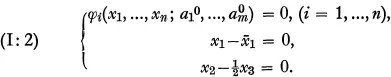
We begin with the parameters in the model (I: 1) having the values a_j⁰ and the endogenous variables consequently the values x_i⁰. Let us set up, for example, two economic ends, which we wish to be realized, namely x₁ =

₁ and x₂ =

x₃. With the given parameter values we assume that these ends are not obtained. The task thus consists of changing one or more of the parameter values in such a way that the new restrictions we have placed on x₁, x₂ and x₃ are satisfied. In this way x₂, …, x_n will take on values different from x₂⁰, …, x_n⁰, but as the ends only comprise x₁ and the relation between x₂ and x₃ this is of no importance. The question is now which and how many parameters one may choose as means and which changes in the chosen parameters must be made to achieve the desired result.

Intuitively we may be led to the conclusion that as a rule we are obliged to introduce changes in exactly the same number of parameters as the number of ends. This result follows from the idea that the number of equations and the number of unknowns ought to be equal if the system is to have a definite solution. Our system is now:

We have now n+2 equations with n unknowns; the system is overdetermined. For that reason two parameters may therefore be considered as unknown; thus the number of unknowns and the numbe...

Table of contents

• Cover Page
• Half Title page
• Public Economics
• Title Page
• Copyright Page
• Original Title Page
• Original Copyright Page
• Preface
• Contents
• Introduction
• Part I. General Theory of Fiscal Policy Problems and Methods
• Part II. Micro-Economics of Fiscal Policy The Impact of Fiscal Policy on the Behaviour of Households, Firms and Organizations
• Part III. Macro-Economics of Fiscal Policy Fiscal Policy for Full Employment and a Stable Value of Money
• Index of Authors
• Index of Subjects